Forecasting_CO2_Emissions.pptx

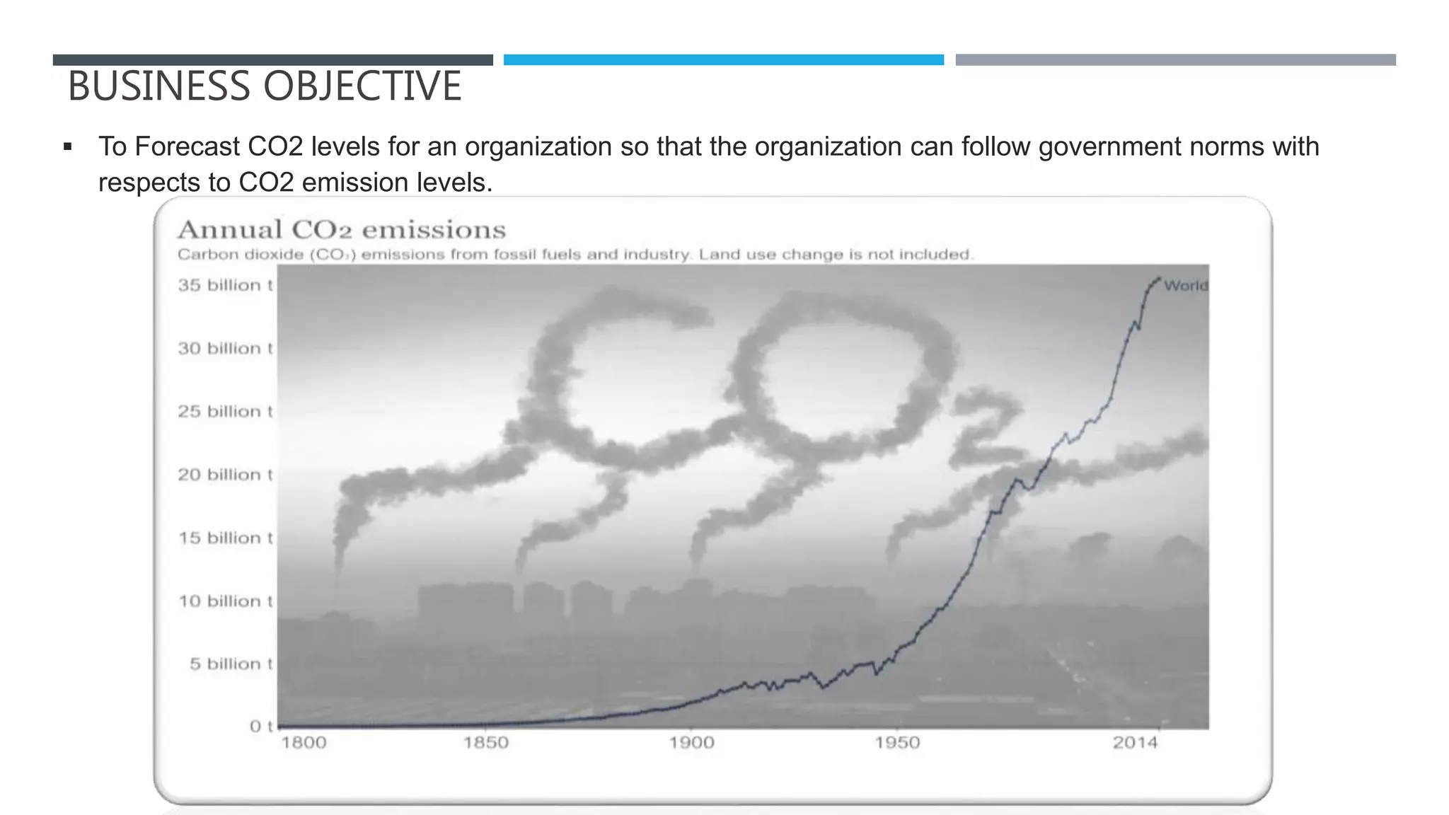
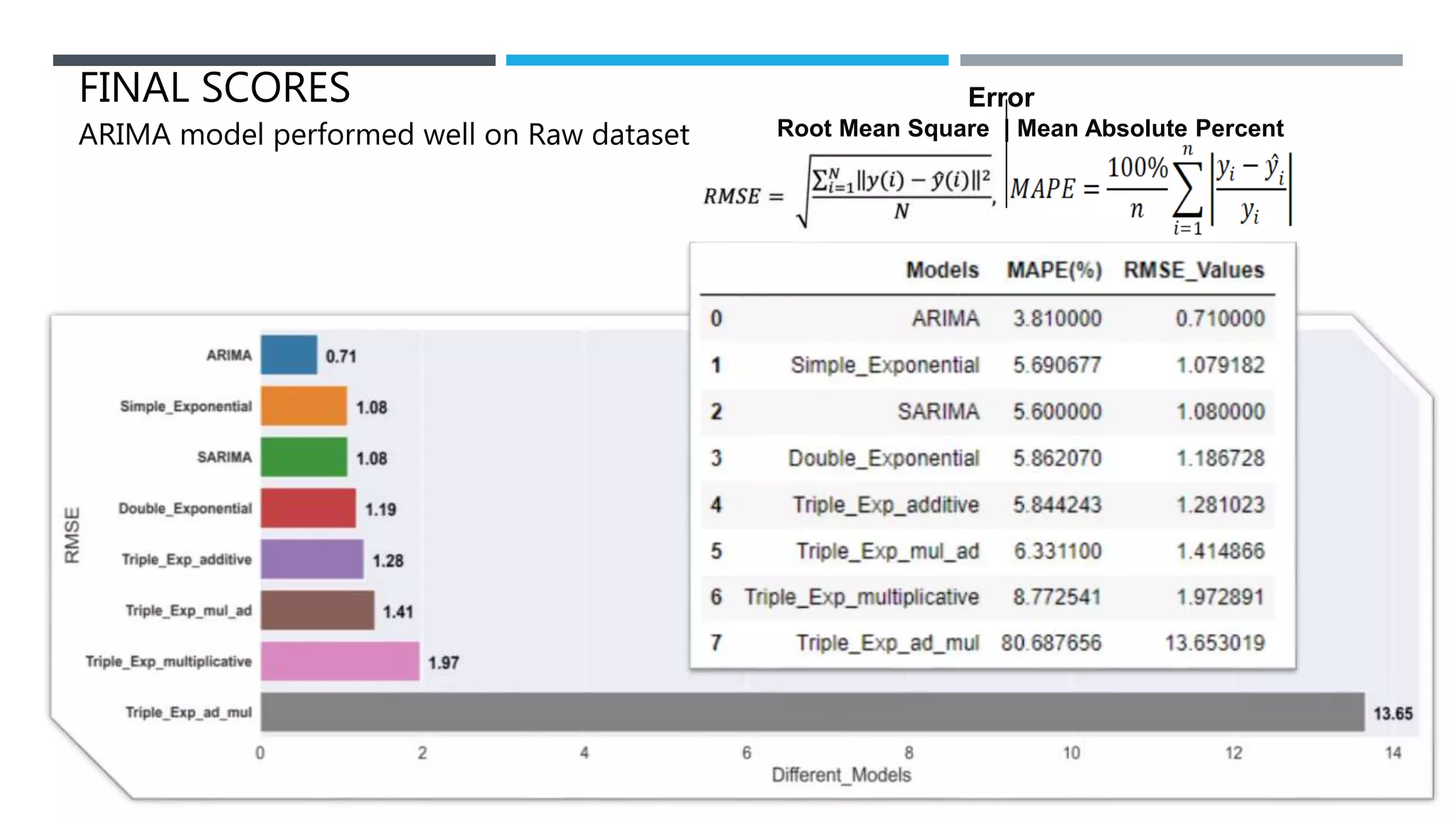
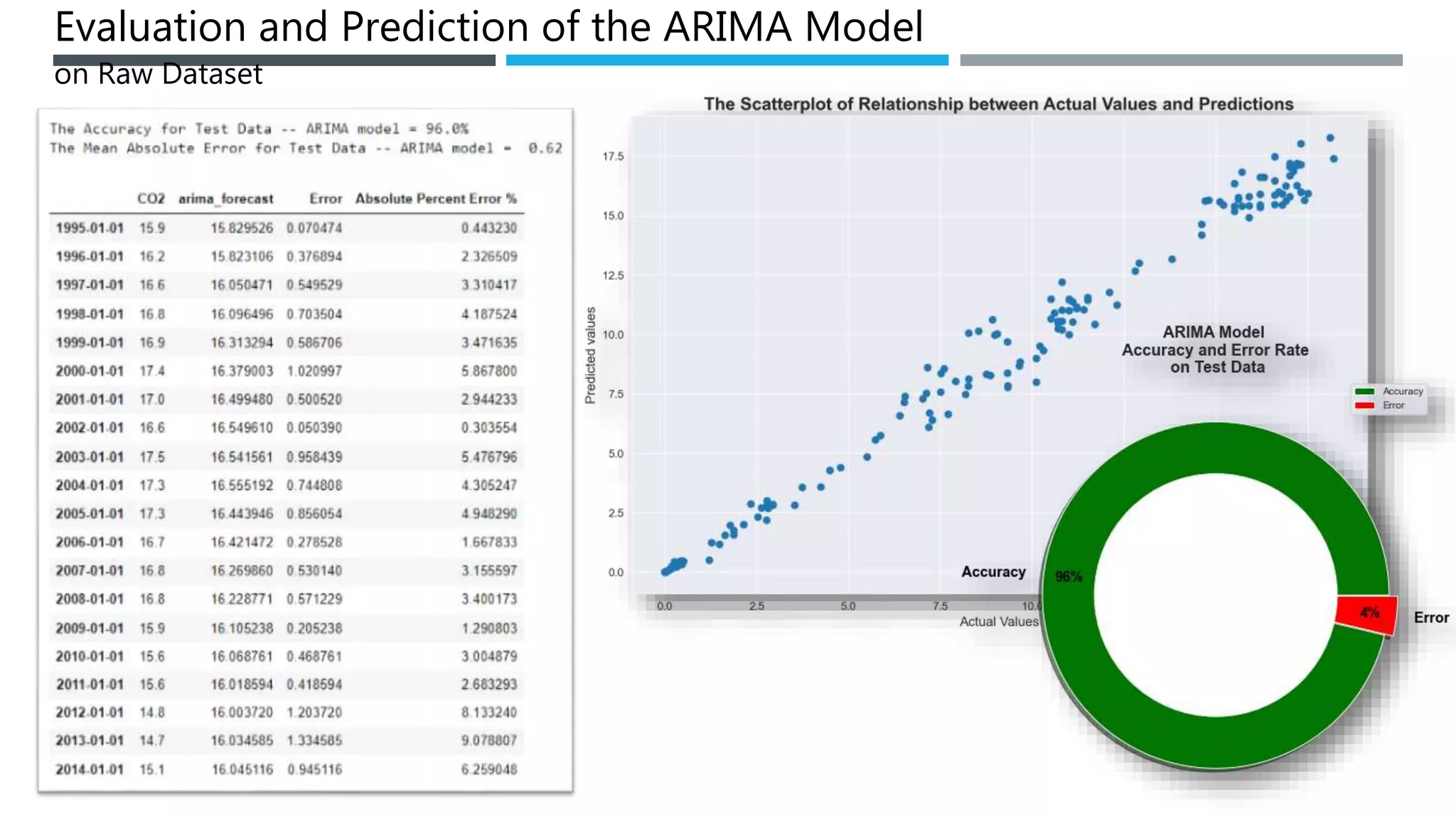
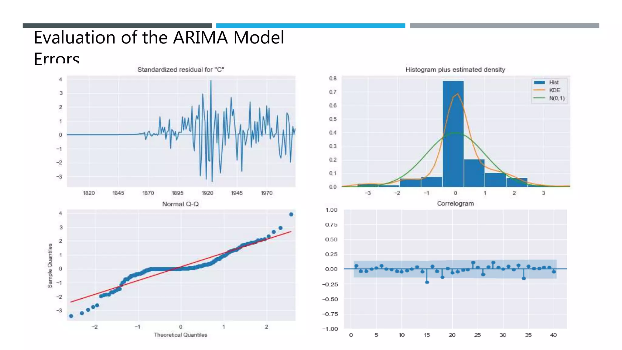
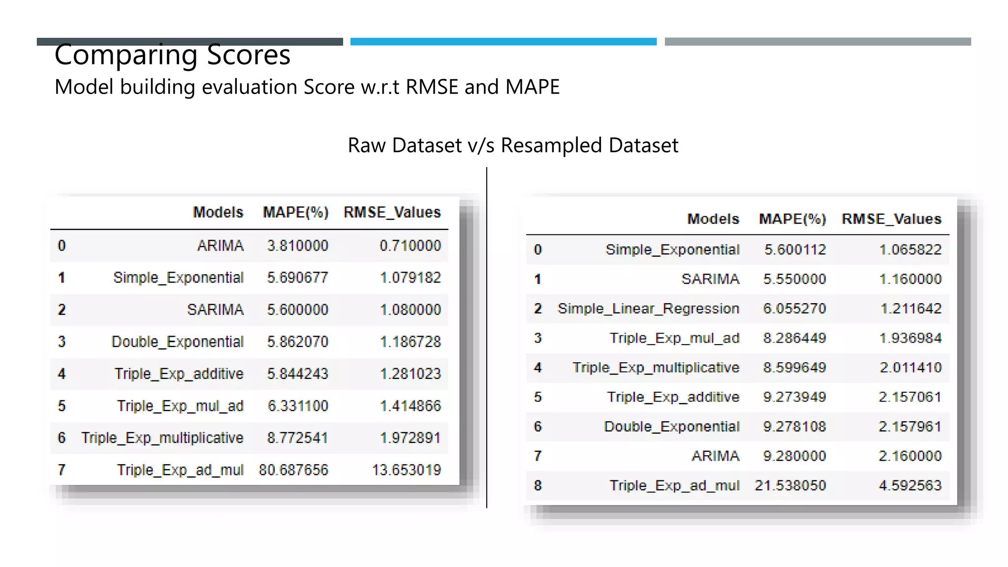
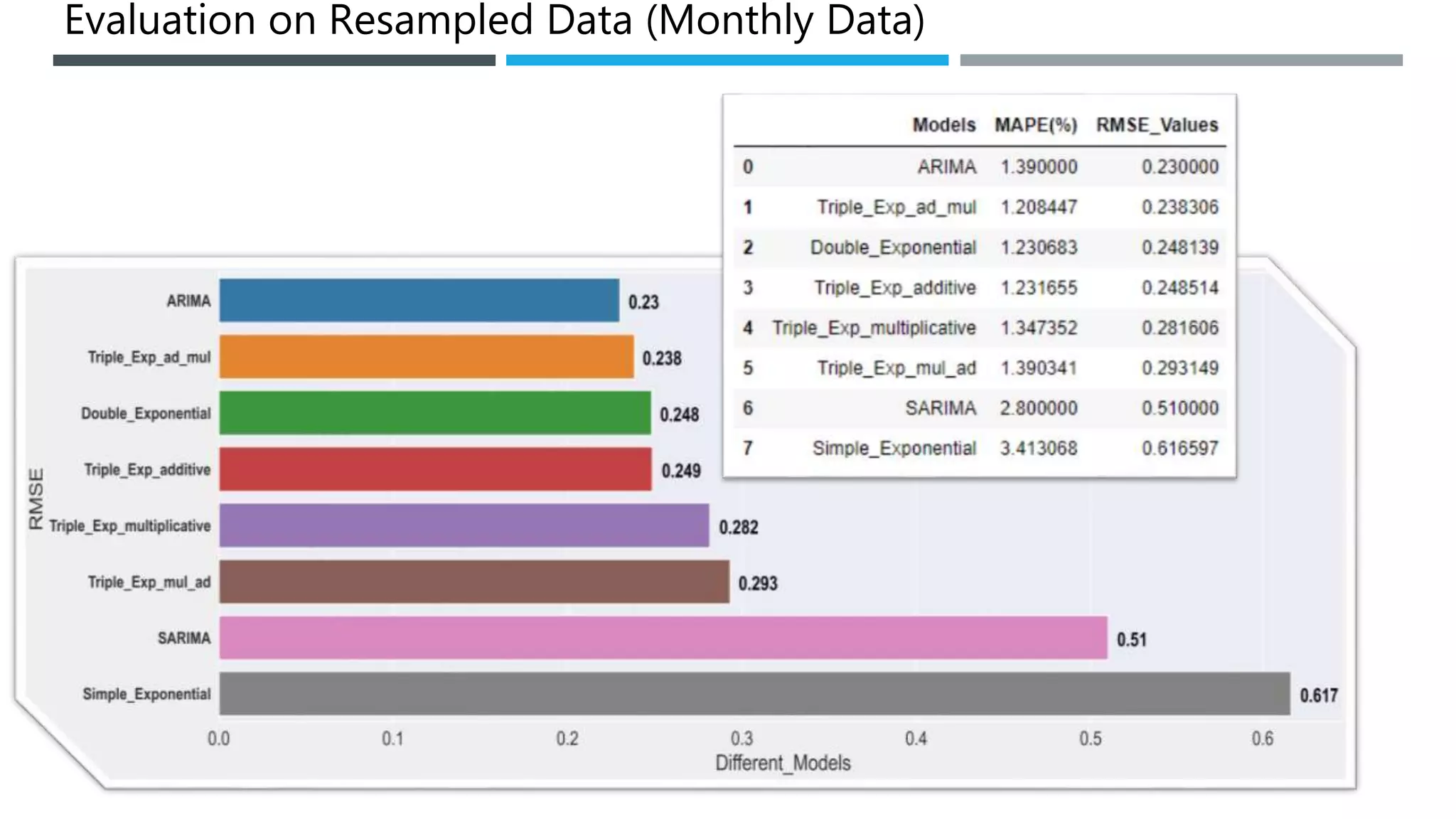
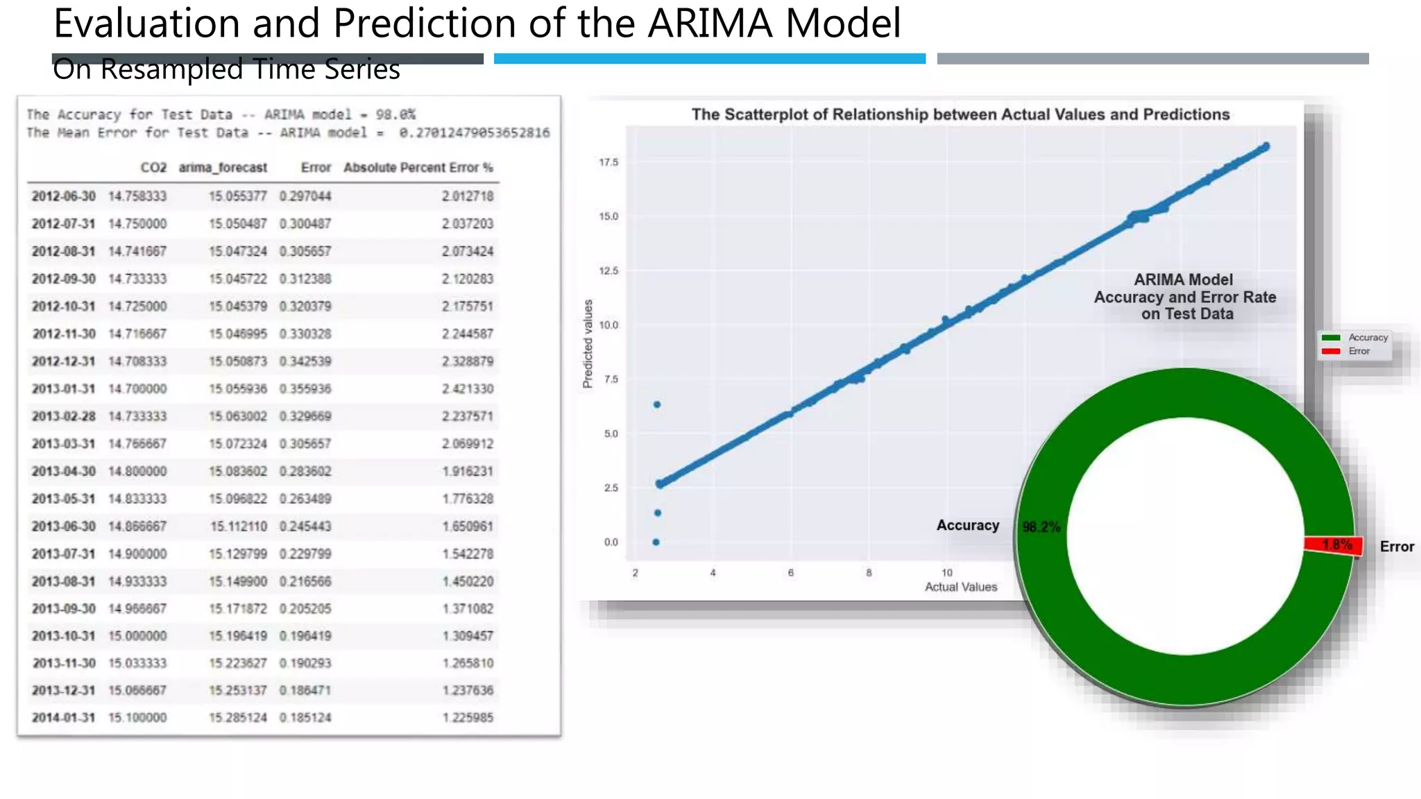
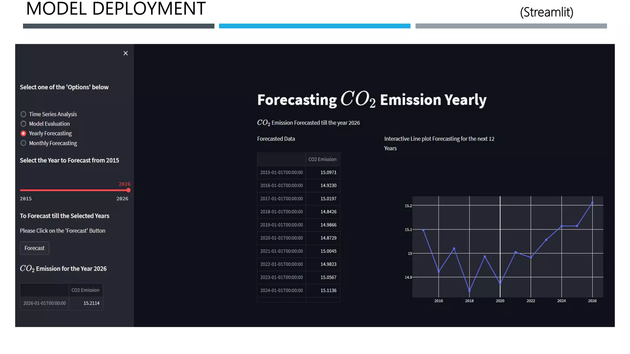
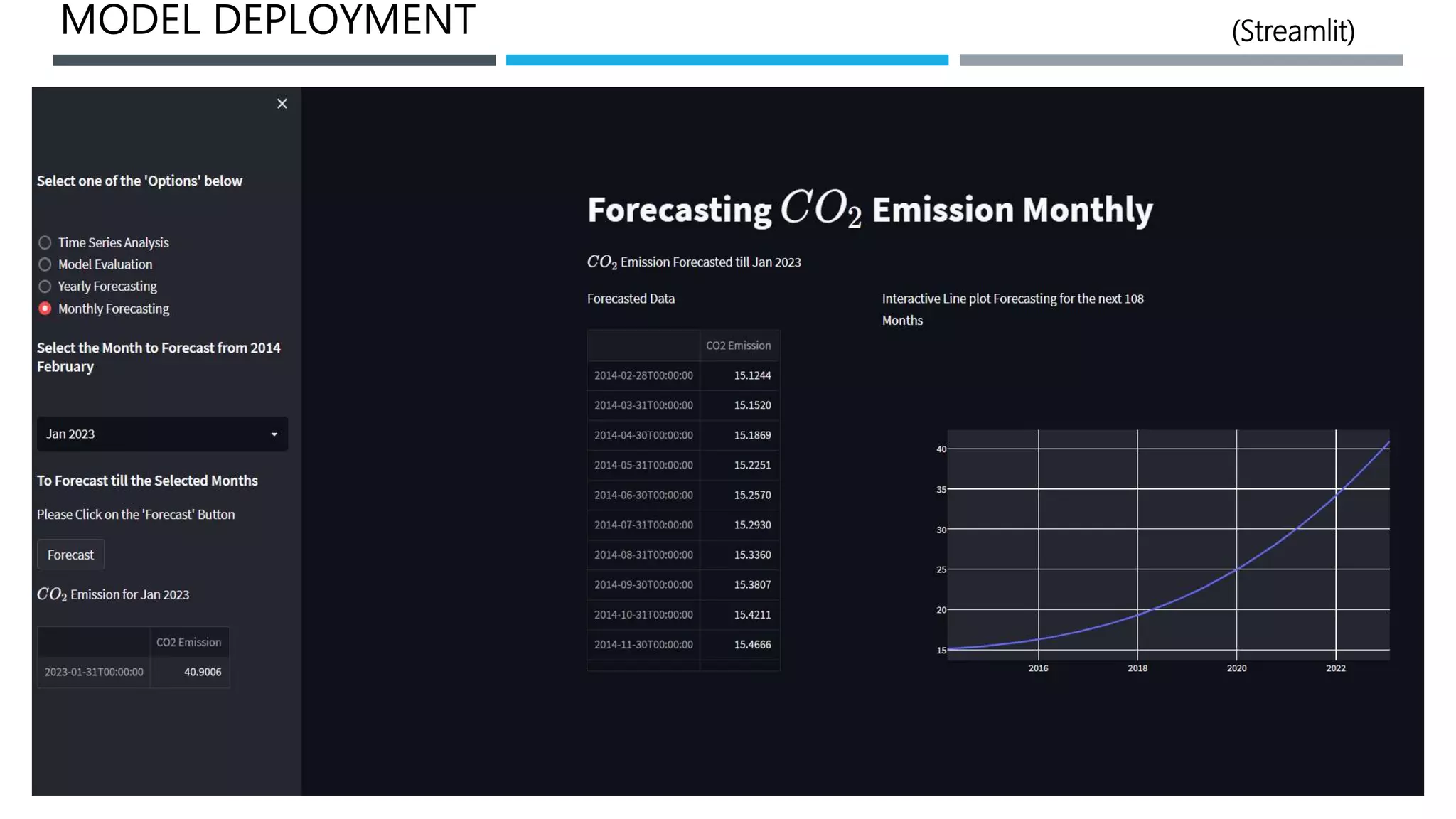
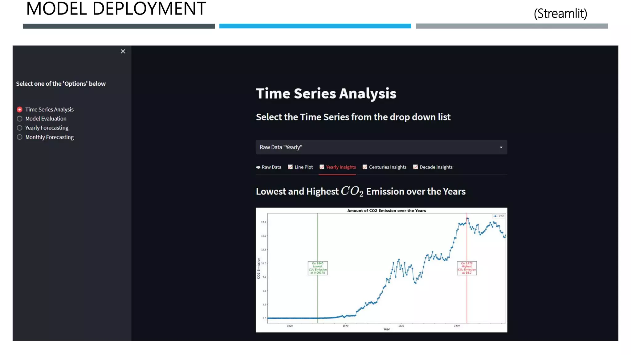
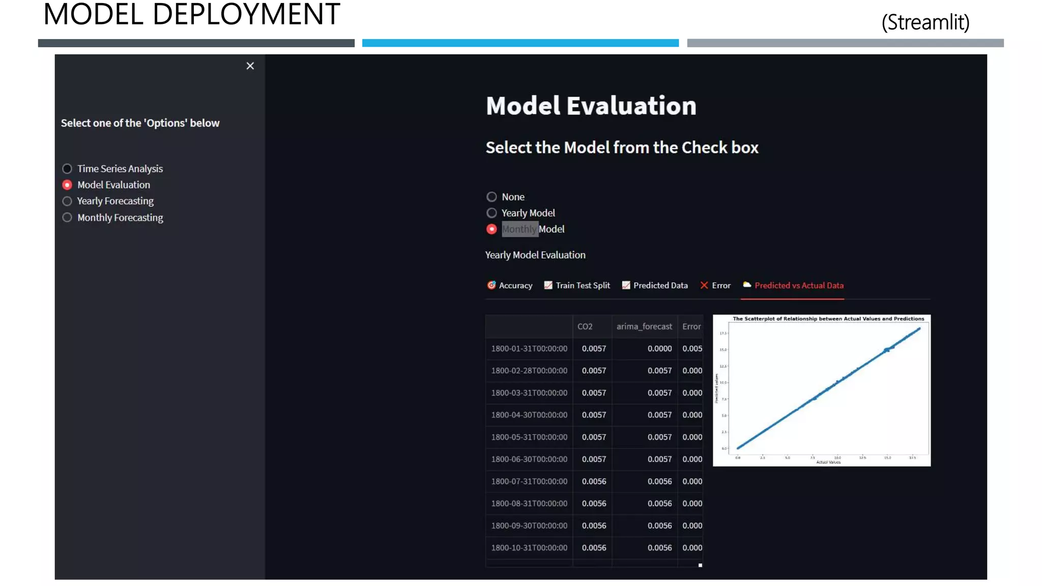
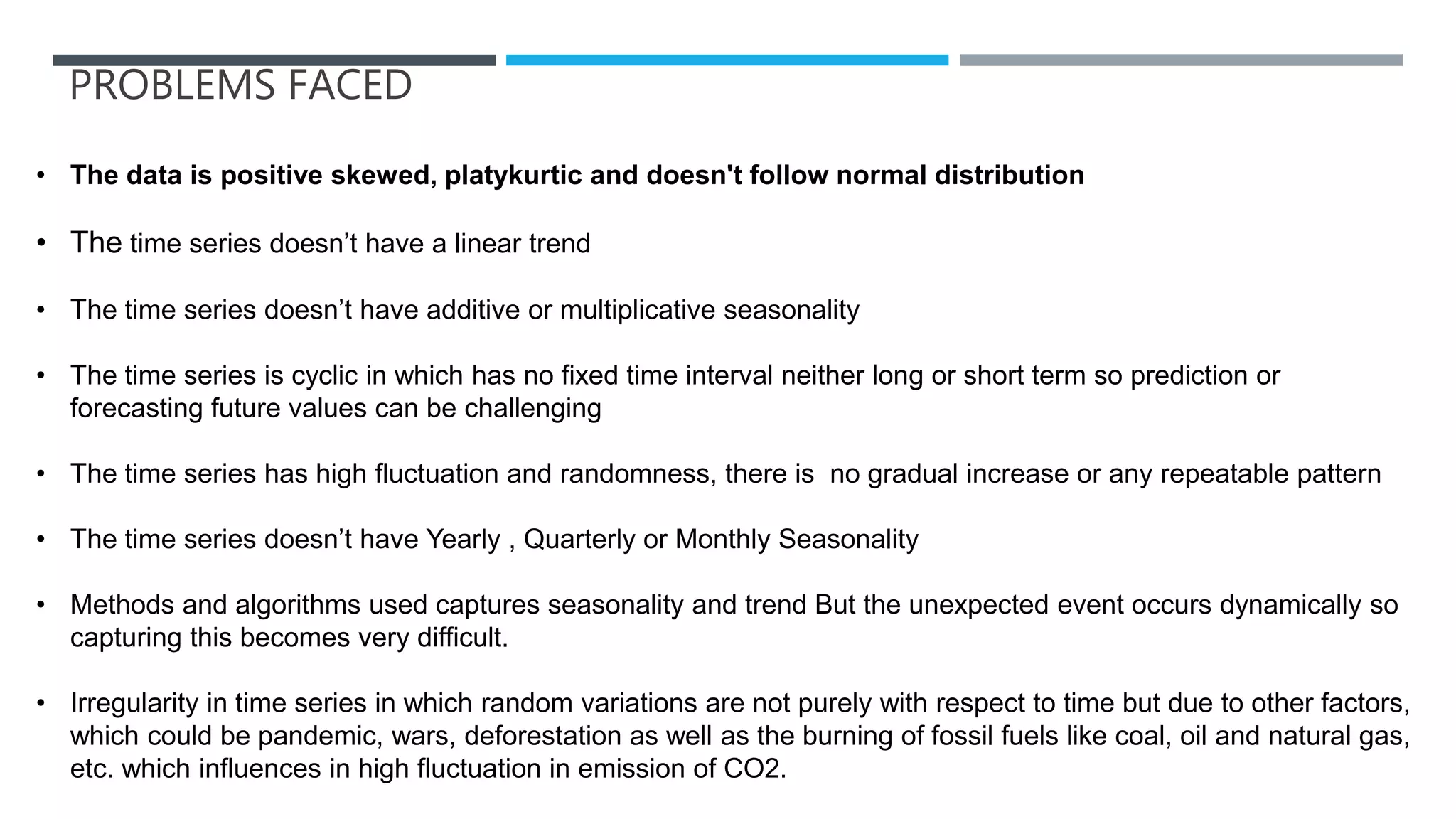
AIR QUALITY FORECASTING
(CO2 EMISSION)
TEAM MEMBERS
1.) MR. MOIN DALVI
2.) MR. ZOHEB KAZI
3.) MR. SOUDAL HODA
4.) MR. SWAPNIL WADKAR
5.) ANAND JAGDALE
6.) ATHIRA RAVI

BUSINESS OBJECTIVE
 To Forecast CO2 levels for an organization so that the organization can follow government norms with
respects to CO2 emission levels.

INTRODUCTION
There is wide consensus among scientists and policymakers that global warming as defined by the
Intergovernmental Panel on Climate Change (IPCC) should be pegged at 1.5 Celsius above the pre-
industrial level of warming in order to maintain environmental sustainability . The threats and risks of climate
change have been evident in the form of various extreme climate events, such as tsunamis, glacier melting,
rising sea levels, and heating up of the atmospheric temperature. Emissions of greenhouse gases, such as
carbon dioxide (CO2) are the main cause of global warming.
In this Project for Time Series Analysis and Forecasting
Each step taken like EDA, Feature Engineering, Model Building, Model Evaluation and Prediction table, and
Deployment. Explaining which model to select on basis of metrics like RMSE, MAPE and MAE value for
each model. Finally explaining which model we will use for Forecasting.
Better accuracy in short-term forecasting is required for intermediate planning for the target to reduce CO2
emissions. High stake climate change conventions need accurate predictions of the future emission growth
path of the participating organization to make informed decisions. Exponential techniques, Linear statistical
modeling and Autoregressive models are used to forecast the emissions and the best model will be selected
on these basis
1.) Minimum error
2.) Low bias and low variance trade off

OUTLIER DETECTION
Observation:
• There are no outliers above the
positive upper extreme whisker.
• There are no outliers below the
negative side of the lower whisker
• The data looks right skewed which
means there are extreme values that do
not follow the regular trend of the data

DATA VISUALIZATION
Observation: As we can observe that approximately after ‘1845’ there is a increase in the
amount of ‘CO2’ Emission and at ‘1979’ it was at its peak.
•There has been a
significant increase in the
amount of ‘CO2’ emission
after ‘1870’.
•With increasing time the
amount of emission of
‘CO2’ is also increasing.
•The lowest ‘CO2’
emission recorded was
‘0.00175’ on ‘1845’
•The highest ‘CO2’ that
was recorded ‘18.2’ on
‘1979’
• We can see there was
an plateau
in ‘CO2’ Emission from
‘1800’ to ‘1860’ not much
of a variance, mostly
constant.

DATA VISUALIZATION
LAG PLOTS (YEARLY)
A lag plot is a special type of
scatter plot in which the X-
axis represents the dataset
with some time units behind
or ahead as compared to the
Y-axis. The difference
between these time units is
called lag or lagged and it is
represented by k.
Observation: Our data is
linear mostly linear and it
shows positive
autocorrelation with the
previous lag values and it
has an underlying
structure of and
autoregressive model.

CORRELATION OF THE DATASET
Observation:
• There is a positive linear correlation between
the independent feature ‘Year’ and the dependent
feature ‘CO2’.

Sampling Yearly into Monthly time series
Interpolation method
Using ‘linear’: You draw a straight line joining the next and previous points of the missing values in the data.

DATA VISUALIZATION
LAG PLOTS (MONTHLY)
Observation: Our data
shows positive linear
autocorrelation with the
previous lag values
(previous months)

TIME SERIES DECOMPOSITION PLOT
Observation:-
1. Observed - Actual data
2. Trend - Increasing trend.
3. Seasonal-
- Does not Varies with the mean 0.
- No seasonality found.
4. Residual - It is the noise pattern of the
time series data for each year, which was
not captured by the two components -
Trend and Seasonality. Residual is the left
over after decomposition of the two major
components (Trend and Seasonality)

FEATURE ENGINEERING
FEATUREEXTRACTION
Feature Extraction for Visualization Data Pre-processing for Model Driven Techniques

DATA VISUALIZATION
Observation: As we can
observe there is Weekly
seasonality in our time series
data analysis.
Every 23rd week of every Year
we can see a spike in CO2
emission in our time series
It does not have Quarterly or
Monthly seasonality through
out the years.

Observation: In daily analysis of 𝐶𝑂2 emission we are getting a constant
variation among all days throughout the Years.
Hence, we can see there is no Daily seasonality or pattern in CO2 emission
DATA VISUALIZATION

TEST OF STATIONARITY
CONVERTING NON-STATIONARY TIME SERIES INTO STATIONARY
Assumptions of ARMA model
1.Data should be stationary – by
stationary it means that the properties of
the series doesn’t depend on the time
when it is captured. A white noise series
and series with cyclic behavior can also be
considered as stationary series.
2.Data should be univariate – ARMA
works on a single variable. Auto-regression
is all about regression with the past values.
Augmented Dicky Fuller Test
Null Hypothesis (H0): The series is not
stationary
p-value > 0.05
Alternate Hypothesis (H1): The series is
stationary
p-value <= 0.05
Differencing
In this method, we compute the difference
of consecutive terms in the series.
Differencing is typically performed to get
rid of the varying mean. Mathematically,
differencing can be written as:
yt‘ = yt – y(t-1)
where yt is the value at a time t
Applying differencing on our series and
plotting the results:
Observation: Finally our data is
stationary as our p-value is less then
0.05 we can reject Null Hypothesis.
Hence, state our time series is
stationary which means it does not
have any trend and seasonality. The
data does not depend on the time
when it is captured.
First Order Differencing {yt = yt – y(t-1)}

SPLITTING THE RAW DATA INTO TRAIN TEST SPLIT
NO RANDOM PARTITION THAT’S BECAUSE THE ORDER SEQUENCE OF THE TIME SERIES SHOULD BE INTACT
IN ORDER TO USE IT FOR FORECASTING.
LEAVING TEST DATA WITH 5 YEARS OF TIME SERIES
FOR TRAINING AND TESTING WE ARE GOING TO FORECAST FOR THE LAST 5 YEARS. THAT IS FROM 1994 TO 2014.

MODEL BUILDING on Raw Data (Yearly Data)

ARIMA Model Building on (Yearly Data)
ARIMA Hyperparameter Tuning order(p,d,q)
p = Periods to lag for eg: (if P= 4 then we
will use the four previous periods of our
time series in the autoregressive portion of
the calculation) d = In an ARIMA model we
transform a time series into stationary
one(series without trend or seasonality)
using differencing. D refers to the number
of differencing transformations required by
the time series to get stationary.
q = This variable denotes the lag of the
error component, where error component
is a part of the time series not explained by
trend or seasonality.

ARIMA Model Building on (Yearly Data)
Test Data vs Forecasted Data

SARIMA Model Building on (Yearly Data)

SARIMA Model Building on (Yearly Data)
Test Data vs Forecasted Data

FINAL SCORES
ARIMA model performed well on Raw dataset
Error
Root Mean Square | Mean Absolute Percent

Evaluation and Prediction of the ARIMA Model
on Raw Dataset

Evaluation of the ARIMA Model
Errors

Forecasting for the Next 5 Years
Using the ARIMA Model on the Whole Dataset

Comparing Scores
Model building evaluation Score w.r.t RMSE and MAPE
Raw Dataset v/s Resampled Dataset

SPLITTING THE RESAMPLED TIME SERIES INTO TRAIN TEST SPLIT
NO RANDOM PARTITION THAT’S BECAUSE THE ORDER SEQUENCE OF THE TIME SERIES SHOULD BE INTACT
IN ORDER TO USE IT FOR FORECASTING.
LEAVING TEST DATA WITH 5 YEARS OF TIME SERIES
FOR TRAINING AND TESTING WE ARE GOING TO FORECAST FOR THE LAST 5 YEARS. THAT IS FROM 2010 TO 2014.

Evaluation on Resampled Data (Monthly Data)

Evaluation and Prediction of the ARIMA Model
On Resampled Time Series

PROBLEMS FACED
• The data is positive skewed, platykurtic and doesn't follow normal distribution
• The time series doesn’t have a linear trend
• The time series doesn’t have additive or multiplicative seasonality
• The time series is cyclic in which has no fixed time interval neither long or short term so prediction or
forecasting future values can be challenging
• The time series has high fluctuation and randomness, there is no gradual increase or any repeatable pattern
• The time series doesn’t have Yearly , Quarterly or Monthly Seasonality
• Methods and algorithms used captures seasonality and trend But the unexpected event occurs dynamically so
capturing this becomes very difficult.
• Irregularity in time series in which random variations are not purely with respect to time but due to other factors,
which could be pandemic, wars, deforestation as well as the burning of fossil fuels like coal, oil and natural gas,
etc. which influences in high fluctuation in emission of CO2.

Forecasting_CO2_Emissions.pptx

Forecasting_CO2_Emissions.pptx

More Related Content

Similar to Forecasting_CO2_Emissions.pptx

Recently uploaded

Forecasting_CO2_Emissions.pptx