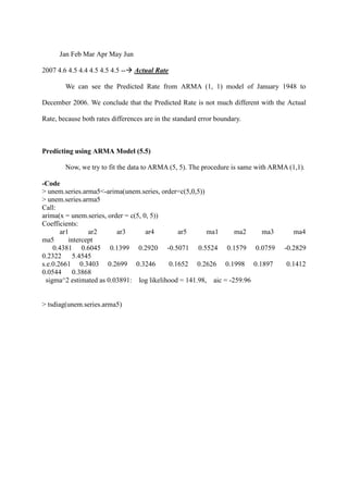
This document discusses using the Box-Jenkins methodology to forecast unemployment rates in the US from January 2007 to July 2007 using past data from January 1948 to December 2006. It first provides an overview of the Box-Jenkins methodology and its key steps: identification, estimation, diagnostics, and forecasting. It then applies these steps using R: identifying an ARIMA(1,1) model as best fitting the deseasonalized data based on minimizing the AIC, estimating the parameters of this model, and selecting ARIMA(1,1) to forecast future unemployment rates.

1. SUNY AT STONYBROOK
Analysis Unemployment Rate by
Box-Jenkins Method Using
R program
AMS 316(Time Series Analysis) Project
Byung Chul Yea
(#105719401)
2010-04-02

2. INTRODUCTION
This project is for forecasting of U.S unemployment rate from January 2007 to July
2007 based on the past long-term data from January 1948 to December 2006. I will use the R
program in all procedure following the Box-Jenkins methodology. First, I will state what the
Box-Jenkins Methodology is. Second, I will develop each procedure of this methodology by
using R and will execute this R code.
1. Box-Jenkins Methodology.
Box-Jenkins Methodology is a general strategy for time-series forecasting, which emphasizes
the importance of identifying an appropriate model in an iterative way. Furthermore Box and
Jenkins showed how the use of differencing can extend ARMA models to ARIMA models
and hence cope with non-stationary series. In addition, they show how to incorporate
seasonal terms into seasonal ARIMA (SARIMA) models. Because of all these fundamental
contributions, ARIMA models are often referred to as Box-Jenkins models. The main stages
in setting up a Box-Jenkins forecasting model are as follow:
2. Procedure.
1.1 Box-Jenkins Model Identification
It consists to determine the adequate model from ARIMA family models. The most general
Box-Jenkins model includes difference operators, autoregressive terms, moving average
terms, seasonal difference operators, seasonal autoregressive terms, and seasonal moving
average terms. First, to Identify an appropriate ARIMA model, the first step in this procedure
is to difference the data until they are stationary.
<Stationarity in Box-Jenkins Models>
1. Constant mean.
2. Constant variance.
3. Constant autocorrelation structure.
This is achieved by examining the correlograms of various differenced series until one is
found that comes down to zero fairly quickly and from which an y seasonal cyclic effect has
been largely removed. However, since we will use R program and this program provides
function „stl‟, I do not need to use differencing method. The function „stl‟ decompose the data

3. into trend term, seasonal term and residual term. Thus, we can remove trend or seasonal
terms easily by using this function instead of differencing method. After removing non-
stationary factor, we obtain stationary data values.
Then, we should decide which the order of ARIMA model is fitted to this data. Akaike‟s
Information Criterion (AIC) is the most commonly used model selection statistics. That is
given (approximately) by:
AIC = −2 ln maximum likelihood + 2r
where r denotes the number of independent parameters that are fitted for that model being
assessed. Thus the AIC essentially choose the model with the best fit, as measured by the
likelihood function, subject to a penalty term, to prevent over-fitting, that increases with the
number of parameters in the variance is included as a parameter. By choosing the r which
minimizes AIC value, we can find the best fitted ARIMA model.
1.2 Box-Jenkins Model Estimation
The main approaches to fitting Box-Jenkins models are non-linear least squares and
maximum likelihood estimation. Maximum likelihood estimation is generally the preferred
technique.
1.3 Box-Jenkins Model Diagnostics
Model diagnostics for Box-Jenkins models is similar to model validation for non-linear least
squares fitting. Model diagnostics for Box-Jenkins models is similar to model validation for
non-linear least squares fitting.
That is, the error term u is assumed to follow the assumptions for a stationary unvaried
process. The residuals should be white noise (or independent when their distributions are
normal) drawings from a fixed distribution with a constant mean and variance.
If the Box-Jenkins model is a good model for the data, the residuals should satisfy these
assumptions. If these assumptions are not satisfied, we need to fit a more appropriate model.
That is, we go back to the model identification step and try to develop a better model.
Hopefully the analysis of the residuals can provide some clues as to a more appropriate
model. The residual analysis is based on:
1. Random residuals: the Box-Pierce Q-statistic: Q(s) = nΣr(k)2 ≈ χ 2 (s) where r(k)
is the k-th residual autocorrelation and summation is over first autocorrelations.

4. 2. Fit versus parsimony: the Schwartz Bayesian Criterion (SBC):
SBC = ln{RSS/n} + {p+d+q}ln(n)/n, where RSS is residual sum of squares, n is
sample size, and (p+d+q) is the number of parameters.
1.4 Forecasting
Suppose we have an observed time series X1, X2, Xn. Then the basic problem is to estimate
future value such as X(n+h), where to integer h is called the lead time or forecasting horizon –h
for horizon. For example, ARMA (1, 1)
ARMA 1,1 Xt − φXt−1 = μ + θZt−1 + Zt −1 < 𝜃 < 1, −1 < 𝛿 < 1 Zt ~N(0, δ)
1 − Step Xn 1 = E Xn+1 X1, … . Xn) = E φXn + Zn+1 + θZn + μ X1, … . Xn)
= μ + φXn + θZn
2 − Step Xn 2 = E Xn+2 X1, … . Xn) = E φXn + Zn+2 + θZn+1 + μ X1, … . Xn)
= μ + φXn(1)
In R, we can execute this procedure using function „predict‟.

5. <Practical time series analysis using R program>
From now, we start analyze the data, using U.S monthly unemployment rate from January
1948 to July 2007. This data is from the Federal Reserve Bank of St. Louis.
<http://www.ams.sunysb.edu/˜xing/statfinbook/ BookData/Chap05/m us unem.txt> We will
analyze the data with the statistic program R.
Code:
>series<-read.table("m_us_unem.txt",skip=1,header=T)
>series
>unem<-ts(series[1:708,2], freq=12, start=c(1948, 1))
>unem
>ts.plot(unem)
Figure 1. U.S. monthly unemployment rates from January 1948 to July 2007
As we can see in the Figure 1, this time series data look it is not stationary. We can
see there is seasonal effect which the value fluctuate up and down repeatedly, and the trend
effect by there is no constant mean. In this condition (non-stationary), we cannot use this data
to forecast future value. We need to do differencing process to remove trend effect and
seasonal effect.
Time
unem
1950 1960 1970 1980 1990 2000
46810

6. (a) Plot the ACF of the rates and the 1-lag difference of the rates.
-Plot the ACF of the rates
Code
>par(mfrow=c(2,1))
>acf(unem);pacf(unem)
Figure 2 ACF (top panel) and PACF (bottom panel) of the unemployment rate.
We can distinguish whether the plot is stationary or not through the Autocovariance
Function (ACF) or Partial Autocovariance Function (PACF). Non-stationary series have an
ACF that remains significant for half a dozen or more lags, rather than quickly declining to
zero. We must difference such a series until it is stationary before you can identify the
process. In the ACF graph, the values look decreasing exponentially. It means that the time
0.0 0.5 1.0 1.5 2.0
0.00.40.8
Lag
ACF
Series unem
0.0 0.5 1.0 1.5 2.0
-0.20.41.0
Lag
PartialACF
Series unem

7. series is not stationary. We will fix the time series model to the adaptable form in the next
procedure.
.
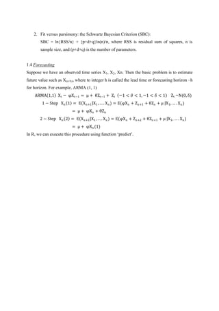
-Code for The 1-lag difference of the rates
>a<-diff(unem,lag=1)
>ts.plot(a)
>a
Figure 3. 1-lag difference of the rates
Comparing to Figure 1, Figure 3 which is 1-lag difference data looks stationary
which means that the mean of the data is constant, and the variance also looks more stable
than Figure 1. Now, it is acceptable data to use Box Jenkins procedure.
(b)Fit ARMA(1,1) model to the data from January 1948 to Dec. 2006
-Code for Seasonal, Trend, remainder
Unem.stl<-stl(unem, “periodic”)
Names(unem.stl)
Unem.stl$time
>par(mfrow=c(3,1))
>plot(unem.stl$time[,2]); # trend
>plot(unem.stl$time[,1]); # seasonal
Time
a
1950 1960 1970 1980 1990 2000
-1.5-1.0-0.50.00.51.0

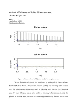
8. > plot(unem.stl$time[,3]); # residual
Figure 4: trend, seasonal effect, and residual
Figure 4 is decomposed data of unemployment rate. The first plot is the trend of the time
series of unemployment rate, second is the seasonal effect, and the last one is the residuals.
Through these plots we can decide that this data has weak seasonal effect, but we cannot see
the trend effect. We will use the trend component value and residuals values for forecasting.
We fit an ARMA model to the deseasonalized series Xt, which consists of the trend and the
residuals.
-Code for deseasonalized time series from the training
>unem.series <-unem.stl$time[,2]+unem.stl$time[,3]
Time
unem.stl$time[,2]
1950 1960 1970 1980 1990 2000
46810
Time
unem.stl$time[,1]
1950 1960 1970 1980 1990 2000
-0.0100.005
Time
unem.stl$time[,3]
1950 1960 1970 1980 1990 2000
-0.50.5

9. > par(mfrow=c(2,1))
> acf(unem.series); pacf(unem.series)
Figure 5. ACF (top panel) and PACF (bottom panel) of the deseasonalized time series.
We draw the ACF and PACF graph again without the trend effect. Comparing to
figure 2, the values more exponentially, smoothly decrease as time goes by. These data will
be fitted in ARMA model through the result of checking ACF function. To find the order of
AR and MA, we can use the AIC criteria from (1, 1) to (5, 5).
Let us see the result by running two models. (ARMA (1, 1) and ARMA (5, 5))
-Code for ARMA (1, 1)
aic<-matrix(rep(0,25), 5, 5);
for(i in 1:5) for (j in 1:5){
fit.arima<-arima(unem.series, order=c(i,0,j))
aic[i,j]<-fit.arima$aic}

10. aic
> aic
[,1] [,2] [,3] [,4] [,5]
[1,] -166.6036 -207.9955 -219.1004 -230.7408 -247.3997
[2,] -225.4142 -257.7890 -214.1998 -221.8776 -257.1761
[3,] -254.9962 -256.2421 -261.3230 -274.9241 -259.6045
[4,] -254.4048 -261.5649 -259.3315 -255.3169 -256.1432
[5,] -252.8203 -258.3666 -265.0479 -254.8651 -259.9598
The ACF and PACF of the deseasonalized series are plotted in Figure 5, which shows
significant autocorrelations for lags. We fit an ARMA model to the deseasonalized series by
using the AIC to determine the order of the ARMA model. We select the model that gives us
the minimum AICs. Now, to predict standard error, it needs to be plugged into ARMA model.
ARMA (1, 1) model is minimum absolute value. Thus we take ARMA (1, 1) as fitted model.
Based on the AIC, we fit the ARMA (1, 1) model with the standard errors of the parameter
estimates. As you can see, after deseasonalizing the time series of unemployment rates,
finally it fully satisfies the stationary condition. Before we go onto next step, it needs a
hypothesis that if we select higher ARMA model such as ARMA (5, 5), the result (predicted
error) will be more accurate.
-Code
> unem.series.arma1<-arima(unem.series, order=c(1,0,1))
> unem.series.arma1
Call:
arima(x = unem.series, order = c(1, 0, 1))
Coefficients:
ar1 ma1 intercept
0.9889 0.0654 5.3256
s.e. 0.0053 0.0309 0.6906
sigma^2 estimated as 0.0455: log likelihood = 87.3, aic = -166.6
>tsdiag(unem.series.arma1)

11. Figure6. Standardized residuals, ACF of residuals and p-value of Ljung-Box statistics
If a model has been fitted to a time series, we should check that the model really does
represent an appropriate description of the data which is called Model checking. It is very
important, and the assessment of residual is an essential step in verification of the model. In
adequate model, the residuals should be random. If it is dependent on each other, it shows
this model does not completely represent time series components in data and remain certain
data in residual. Then it is necessary to go back to mode selection and try to fit the data into a
better model. To analysis residuals, we plot residuals as a time series, find ACF and calculate
P-value for Ljung-Box statistics using function „tsdiag‟.
As you can see the figure6, Diagnostic of residuals (observation-fitted value) are just
noise (random and close to zero).
Standardized Residuals
Time
1950 1960 1970 1980 1990 2000
-606
0.0 0.5 1.0 1.5 2.0
-0.20.6
Lag
ACF
ACF of Residuals
2 4 6 8 10
0.00.6
p valuesfor Ljung-Box statistic
lag
pvalue

12. (c) Use your fitted model to compute k-months-ahead forecasts (k = 1, 2, . . . , 6) and
their standard errors, choosing December 2006 as the forecast origin. Compare your
forecasts with the actual unemployment rates.
Finally, I predict the value of 2007 and compare with real observation data.
We found the most adequate function to predict future unemployment rate. We can use the
fitted ARMA (1, 1) model to know 6- months-ahead forecasts.
-Code
>unem.pred<-predict(unem.series.arma1, n.ahead=6)
>unem.pred
$pred
Jan Feb Mar Apr May Jun
2007 4.503905 4.513061 4.522115 4.531068 4.539922 4.548677
$se
Jan Feb Mar Apr May
2007 0.2133059 0.3099469 0.3814630 0.4403011 0.4910647
Jun
2007 0.5360747
> unem.pred$pre+ unem.stl$time[1:6,1]
Jan Feb Mar Apr May Jun
2007 4.499849 4.511939 4.527317 4.534397 4.536292 4.560540 -- Predicted Rate
> unem<-ts(series[1:715,2], freq=12, start=c(1948, 1))
>
> ts(series[709:714,2], freq=12, start=c(2007,1))

13. Jan Feb Mar Apr May Jun
2007 4.6 4.5 4.4 4.5 4.5 4.5 -- Actual Rate
We can see the Predicted Rate from ARMA (1, 1) model of January 1948 to
December 2006. We conclude that the Predicted Rate is not much different with the Actual
Rate, because both rates differences are in the standard error boundary.
Predicting using ARMA Model (5.5)
Now, we try to fit the data to ARMA (5, 5). The procedure is same with ARMA (1,1).
-Code
> unem.series.arma5<-arima(unem.series, order=c(5,0,5))
> unem.series.arma5
Call:
arima(x = unem.series, order = c(5, 0, 5))
Coefficients:
ar1 ar2 ar3 ar4 ar5 ma1 ma2 ma3 ma4
ma5 intercept
0.4381 0.6045 0.1399 0.2920 -0.5071 0.5524 0.1579 0.0759 -0.2829
0.2322 5.4545
s.e.0.2661 0.3403 0.2699 0.3246 0.1652 0.2626 0.1998 0.1897 0.1412
0.0544 0.3868
sigma^2 estimated as 0.03891: log likelihood = 141.98, aic = -259.96
> tsdiag(unem.series.arma5)

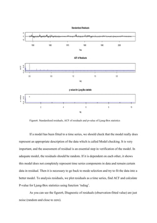
14. Figure7. Diagnostic plots for the fitted ARMA (5, 5) model.
Figure 7 shows us that diagnose residuals (observation-fitted value) are just noise
(random and close to zero) by checking ACF plot. Furthermore, P-value for Lung – Box
Statistics is placed almost around 1. P-value for Lung-Box statistic is also greater than
standard. It indicates that higher level of ARMA model such as ARMA(5, 5) represent more
accurate result. So, we can predict the future unemployment rates 6 month ahead.
-Code
> unem.pred<-predict(unem.series.arma5, n.ahead=6)
> unem.pred
$pred
Jan Feb Mar Apr May Jun
2007 4.468035 4.475790 4.468911 4.516420 4.511021 4.550652
$se
Jan Feb Mar Apr May Jun
2007 0.1972530 0.2776295 0.3643634 0.4499888 0.5339693 0.6232356
> unem.pred$pre+unem.stl$time[1:6,1]
Jan Feb Mar Apr May Jun
Standardized Residuals
Time
1950 1960 1970 1980 1990 2000
-606
0.0 0.5 1.0 1.5 2.0
0.00.8
Lag
ACF
ACF of Residuals
2 4 6 8 10
0.00.6
p valuesfor Ljung-Box statistic
lag
pvalue

15. 2007 4.463979 4.474668 4.474114 4.519748 4.507390 4.562515-Predicted
Rate
> unem<-ts(series[1:715,2], freq=12, start=c(1948,1))
> ts(series[709:714,2], freq=12, start=c(2007,1))
Jan Feb Mar Apr May Jun
2007 4.6 4.5 4.4 4.5 4.5 4.5-- Actual Rate
The result above gives the forecast values of the time series from January to June
2007 based on the ARMA(5, 5) model of January 1948 to December 2006 unemployment
rate. Finally, we obtained the future value from analyzing past data. To check all the
procedures worked successfully, we compare the predicted value to real value. The Predicted
Rate is not much different with the Actual Rate in ARMA(5, 5), because both rates
differences are in the standard error boundary. Thus, I am able to conclude that my prediction
with ARMA (5, 5) is appropriate.
We can conclude that both ARMA (1, 1) and ARMA(5, 5) are acceptable, because the
differences are in the standard error boundary. However, higher ARMA model prediction will
be more accurate than lower ARMA model even though the ARMA(1, 1) is easier to deal
with data.