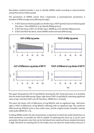
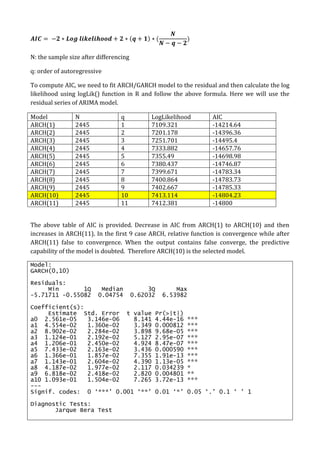
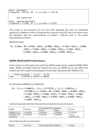
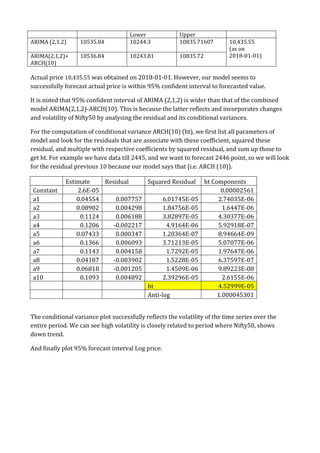
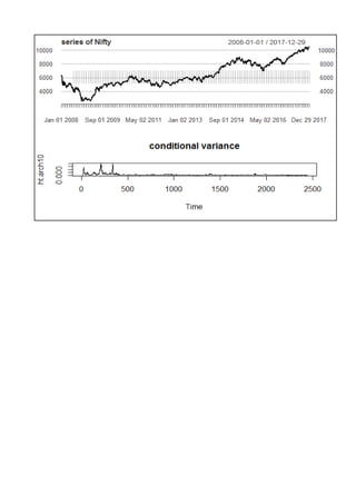
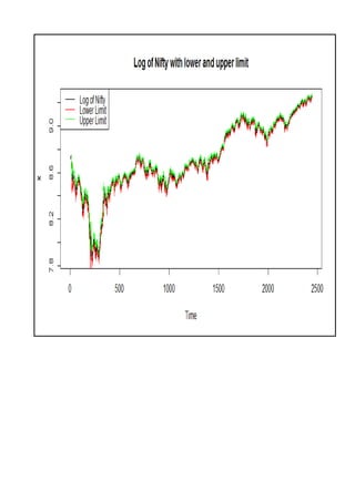
National Institute of Securities Markets (NISM),
Post-Graduation Diploma in Quantitative Finance (PGDQF)
Subject: Financial Time Series Modelling
Project on
Time Series Modelling with ARIMA-ARCH/GARCH
By โ€“ Jeevan A. Solaskar
Introduction:
Forecasting / Predicting or forecasting any financial instrument is always interested topic for
those who are the participant of the financial market. Because of there is directed to the
money they are invested in the market or going to invest the market, as it benefit them. We
are using the time series analysis tool i.e. Autoregressive Integrated Moving Average (ARIMA)
tool for the forecasting the future price movement of National Stock Exchange (NSE), India
index NIFTY 50. NIFTY 50 is the flagship index of NSE. The index tracks behaviour of a
portfolio of blue chip companies, the largest and most liquid Indian securities. It includes 50
of the approximately 1600 companies listed on the NSE, captures approximately 65% of its
float adjusted market capitalization and is true reflection of the Indian stock Market. The
comparison and performance of the ARIMA model have been done using Akaike Information
criteria (AIC) and Maximum likelihood Estimation (MLE). Analysis of prediction is based on
the varying span of historical data.
Time series analysis is concerned with external effect of the irregular component, trend,
seasonality and its own previous lag. This component of time series is using to predict future
with past experience. In the time series, time would serve as the independent variable in the
estimation and other observed variable as the dependent variable. Time series analysis aims
to achieve various objective like, descriptive analysis ( to determine the trend or pattern in a
time series), spectral analysis ( separate periodic or cyclical components), forecasting
(extensively using in business for budgeting based on historical tends), intervention analysis
(event base movement in stock price) and explanative analysis ( correlation between to
stocks). Biggest advantages are that to predict the future.
ARIMA:
Time series forecasting use various statistical principle and concepts to a given historical data
of a variable to forecast future value of same variable. Auto-regression (AR) the values of a
given time series data are regression their own previous lags. Moving Average (MA) is the
nature of the model is representing the error terms. The combination the AR (p) and MA (q) is
called Auto-regressive Moving Average (ARMA (p,q) ) on the stationary data. Here p stands
for order of AR and q for MA. When we combining differencing of the non-stationary time series
with ARMA model called Auto-regressive Integrated Moving Average (ARIMA (p, d, q)). ARMA model
assume the time series is stationary, which is rarely happen. So there is need to remove the
trend, seasonal and noise form the series. Removing the non-stationary part from the data we
have to add in the model, which is done by taking differencing by once, twice etc. until data
series become stationary. In ARIMA modelling latter โ€˜lโ€™ stands for differencing of the series
and denoted by d.
Stationary and differencing of the time series:
1. Stationary:
The first step in the modelling time series data is to covert the non-stationary time series
to stationary one. This is important for the fact a lot of time series model base on the
assumption that stationary time series. Non-stationary time series is unpredictable as it
consist of noise in it on the other hand stationary time series is mean reverting. Stationary
behaviour of time series is mean, variance and correlations are useful for predicting future
behaviour. Example, if the series is consistently increasing over the period, the sample
mean and variance will grow with the sample size, and there will be chance the we will
underestimate mean and variance in the future time period, problem if the mean and
variance of the series are not well defined. In addition, stationary and independence of
random variables are closely related because many theories that hold for independent
random variables also hold for stationary time series in which independence is a required
condition. So what is stationary time series?
Stationary time series shows no long-term trend, has constant mean and variance, if for all
t and t-s.
๐‘ฌ(๐’€๐’•) = ๐‘ฌ(๐’€๐’• โˆ’ ๐’”) = ๐
๐‘ฌ(๐’€๐’• โˆ’ ๐) = ๐‘ฌ(๐’€๐’• โˆ’ ๐’” โˆ’ ๐) = ๐ˆ ๐Ÿ
๐‘ฌ(๐’€๐’• โˆ’ ๐’€๐’• โˆ’ ๐’”) = ๐‘ฌ(๐’€๐’• โˆ’ ๐’‹ โˆ’ ๐’€๐’• โˆ’ ๐’” โˆ’ ๐’‹) = ๐œธ
๐œ‡, ๐œŽ, ๐›พ are constant. ๐›พ0 is equivalent to variance of Yt. A time series is stationary if its mean
and all autocovariance are unaffected by the change in time. This is also called as
covariance stationary and weekly stationary. Another type is strong stationary, process
need not have finite mean and variance. Time series Yt is said to be strict stationary of the
joint distribution of Yt, Yt-1, . . . , Yt-s is the same as the Yt+s, Yt+s+1, . . . , Yt+s+j. In the strict
stationary implies that the probability distribution of time series does not change over
time.
๏‚ท Strict stationary does not imply weak stationary because it does not require finite
variance.
๏‚ท Weak stationary does not imply strict stationarity because higher moments might
depends on time. On the other hand strict stionarity requires probability
distribution does not change over time.
๏‚ท Nonlinear function of strict stationary series, it does not imply to weak
stationarity.
2. Differencing
In order to covert non stationary series to stationary, differencing method can be used in
which the series is lagged 1 step and subtracted from original series.
๐’€๐’• = ๐’€๐’• โˆ’ ๐Ÿ + ๐’†๐’•
๐’†๐’• = ๐’€๐’• โˆ’ ๐’€๐’• โˆ’ ๐Ÿ
In financial time series, it is often that the series is transformed by lagging and then the
differencing is performed. This is because financial time series is usually exposed to
exponential growth and log transformation can smooth out the effect of series and
differencing will help stabilizing the variance of the series.
For the analysis we used R programming and from importing data of Nifty50 adjusted close
used package quantmod. Analysis data points are 736 from 2015-01-01 to 2017-12-31.
The upper left hand side is the original graph of Nifty50, form2015-01-01 to 2017-12-31.
Show the upward movement after Jan 2017. Upper right side is the log transformed graph.
Log transformed graph is more linear compare to original one.
On lower left graph is difference of Nifty50 with its own previous lagged. The level of
variance is high, as series is no stationary. On lower right is side is difference of log
transformed series. This graph is more mean reverting compare to difference graph and
variance is constant.
ARIMA Modelling
1. Model Identification:
Time domain method is established and implemented by observing the autocorrelation of the
time series. Therefore, autocorrelation and partial autocorrelation are the core ARIMA model.
Box-Jenkins method provides a way to identify ARIMA model according to autocorrelation
and partial autocorrelation graph.
The parameters of ARIMA consist three components: p (autoregressive parameter), d
(number of differencing), and q (Moving Average).
๏‚ท If ACF (Autocorrelation graph) cut off after lag n, PACF (partial Autocorrelation) graph
dies down. Then ARIMA (0, d, q). Identify MA(q) process.
๏‚ท If ACF dies down, PACF cut off after lag n, ARIMA (p, d, 0). Identify AR(p) process.
๏‚ท If ACF and PACF die down, mixed ARIMA model and need differencing.
The upper left graph the ACF of Log Nifty50, showing the ACF slowly decreases. It is probably
that the model need differencing. Upper right shows PACF of log Nifty50, indicating significant
value at lag 1 and then PACF cuts off. Therefore, ARIMA (0, 0, 1) model.
The lower left shows, ACF of differences of Log Nifty50, with no significant lags. And lower
right is PACF of differences of log Nifty50, reflecting with no significant lags. The model for
differenced log, Nifty50 series is thus white noise, and the original model resembles random
walk model ARIMA (0, 1, 0).
In fitting ARIMA model, the idea of parsimony is important in which the model should have as
small parameters as possible yet still be capable of explaining the series (p, d, q) the more
parameters the greater noise that can be introduced into model and hence standard deviation
is high. Therefore we checking AIC for the model, once can check for model with p and q are 2
or less. In Box-Jenkins recommend the differencing approach to achieve stationary. However,
primary tools for doing this are the autocorrelation and partial autocorrelation plot. The
sample ACF and PACF plot are compared to the theoretical behaviour of these plots. In
addition to Box-Jenkins method, AIC provides another way to heck and identify the model. AIC
is corrected Akaike Information Criterion and calculated as follows:
๐‘จ๐‘ฐ๐‘ช = ๐‘ป ๐ฅ๐ง(๐’“๐’†๐’”๐’Š๐’…๐’–๐’‚๐’ ๐’”๐’–๐’Ž ๐’๐’‡ ๐’”๐’’๐’–๐’‚๐’“๐’† + ๐Ÿ๐’
Wheren= number of parameters estimated (p + q + possible constant term);
T = number of usable observation.
While considering AIC it is important to note that increasing the number of regressor increase
n, but should have the effect of reducing the residual sum of squares. Thus, if regressor has no
explanatory power, adding it to the model will cause AIC to increase, so marginal cost of
adding regressor is greater. According to AIC method, the model with lowest AIC will be
selected. Based on AIC, we should select ARIMA (2,1,2).
Model (0,1,0) (1,1,0) (0,0,1) (1,1,1) (1,1,2)
AIC -13792.08 -13801.53 -13802.09 -13800.63 -13803
Model (2,1,1) (2,1,2)
AIC -13804.08 -13809.55
2. Parameters estimation:
To estimate the parameters, the result will provide the estimate of each element of the model.
Using ARIMA ( 2,1,2) as selected model, the result is as follows:
Call:
arima(x = log.nifty, order = c(2, 1, 2))
Coefficients:
ar1 ar2 ma1 ma2
1.2482 -0.7747 -1.2011 0.7138
s.e. 0.1676 0.1604 0.1881 0.1778
sigma^2 estimated as 0.000205: log likelihood = 6909.77, aic = -13809.55
the full model:
๐’€๐’• โˆ’ ๐’€๐’•โˆ’๐Ÿ = ๐Ÿ. ๐Ÿ๐Ÿ’๐Ÿ–๐Ÿ(๐’€๐’•โˆ’๐Ÿ โˆ’ ๐’€๐’•โˆ’๐Ÿ) โˆ’ ๐ŸŽ. ๐Ÿ•๐Ÿ•๐Ÿ’๐Ÿ•(๐’€๐’•โˆ’๐Ÿ โˆ’ ๐’€๐’•โˆ’๐Ÿ‘) โˆ’ ๐Ÿ. ๐Ÿ๐ŸŽ๐Ÿ๐Ÿ(๐’†๐’•โˆ’๐Ÿ) + ๐ŸŽ. ๐Ÿ•๐Ÿ๐Ÿ‘๐Ÿ–( ๐’†๐’•โˆ’๐Ÿ) + ๐’†๐’•
3. Diagnostic Checking:
The procedure includes observing residual plot and its ACF and PACF diagram, and check
Ljung-Box result. If ACF and PACF of the model residual show no significant lags, the selected
model is appropriate.
The residual plot, ACF and PACF do not have any significant lag, indicating ARIMA (2,1,2) is a
good model to represent the series.
In addition, Ljung-Box test also provide a different way to double check the model. Ljung-Box
is a test of autocorrelation in which it verifies whether the autocorrelation of a time series are
different from 0. In other words, if the result rejects the hypothesis, this means the data is
independent and uncorrelated. Otherwise, if result rejects the hypothesis, this means the data
is independent and uncorrelated.
Box-Ljung test
data: arima212$residuals
X-squared = 0.7474, df = 1, p-value = 0.3873
Output of Ljung-Box test shows that p-value of the statistics is greater than 0.05, so we are fall
to reject null that the autocorrelation is different from 0. Therefore, the selected model is an
appropriate one for Nifty50.
ARCH/GARCH
Econometric model, the variance of the disturbance term is assumed to be constant. However,
as an asset holder you would be interested in forecasts of the rate of return and variance of
the series. The unconditional variance would be unimportant if you plan to buy the asset at t
and sell at t+1. ARIMA model is linearly model the data and the forecast remain constant
because the model does not reflect recent changes or incorporate new information. It provide
best linearity forecast for the series, and thus forecasting for non-linear model plays little role.
While forecasting non-linear model, ARCH/GARCH model plays an important role.
Residual of ARIMA (2,1,2)
Time
arima212$residuals
0 500 1000 1500 2000 2500
-0.10
0 5 10 15 20 25 30
0.0
Lag
ACF
ACF of ARIMA (2,1,2)
0 5 10 15 20 25 30
-0.04
Lag
PartialACF
PACF of ARIMA (2,1,2)
Check if residual plot displays any kind of cluster of volatility. Next, the squared residual plot.
If there are cluster of volatility, ARCH/GARCH should be should be used for modelling
volatility. And ACF and PACF of the squared residual will help to confirm the noise terms are
not independent and can be predicted. If residual are strict white noise, they are independent
with zero mean, normally distributed, and ACF and PACF of squared residual displays no
significant lags.
Following are the plot of squared residuals:
๏‚ท Squared residual plot shows cluster at some point in time.
๏‚ท ACF seem to die down.โ€™
๏‚ท PACF cut off after lag 10 even though some remaining lags are significant.
ARCH/GARCH is necessary to model the volatility of the series. As indicated by its name,
method shows the conditional variance.
General form of ARCH(q):
๐‘ฌ(๐’‰๐’•
๐Ÿ
| ๐’†๐’•โˆ’๐Ÿ, ๐’†๐’•โˆ’๐Ÿ, โ€ฆ ) = ๐’‚ ๐ŸŽ + ๐’‚ ๐Ÿ ๐’†๐’•โˆ’๐Ÿ
๐Ÿ
The conditional variance of ๐‘’๐‘กis dependent on the realized value of ๐‘’๐‘กโˆ’1
2
. if the realized value
of f ๐‘’๐‘กโˆ’1
2
is large, the conditional variance in t will be large as well. In the above equation, the
conditional variance follows a first order autoregressive process denoted by ARCH (1). In
order to ensure that both ๐‘Ž0 and ๐‘Ž1 have to be restricted. In order to ensure that the
conditional variance is never negative, it is necessary to assume that both are positive. In an
arch model, the error structure is such that the conditional and unconditional means are equal
to zero. ARCH/GARCH orders and parameters are selected based on AIC as follows:
๐‘จ๐‘ฐ๐‘ช = โˆ’๐Ÿ โˆ— ๐‘ณ๐’๐’ˆ ๐’๐’Š๐’Œ๐’†๐’๐’Š๐’‰๐’๐’๐’… + ๐Ÿ โˆ— (๐’’ + ๐Ÿ) โˆ— (
๐‘ต
๐‘ต โˆ’ ๐’’ โˆ’ ๐Ÿ
)
N: the sample size after differencing
q: order of autoregressive
To compute AIC, we need to fit ARCH/GARCH model to the residual and then calculate the log
likelihood using logLik() function in R and follow the above formula. Here we will use the
residual series of ARIMA model.
Model N q LogLikelihood AIC
ARCH(1) 2445 1 7109.321 -14214.64
ARCH(2) 2445 2 7201.178 -14396.36
ARCH(3) 2445 3 7251.701 -14495.4
ARCH(4) 2445 4 7333.882 -14657.76
ARCH(5) 2445 5 7355.49 -14698.98
ARCH(6) 2445 6 7380.437 -14746.87
ARCH(7) 2445 7 7399.671 -14783.34
ARCH(8) 2445 8 7400.864 -14783.73
ARCH(9) 2445 9 7402.667 -14785.33
ARCH(10) 2445 10 7413.114 -14804.23
ARCH(11) 2445 11 7412.381 -14800
The above table of AIC is provided. Decrease in AIC from ARCH(1) to ARCH(10) and then
increases in ARCH(11). In the first 9 case ARCH, relative function is convergence while after
ARCH(11) false to convergence. When the output contains false converge, the predictive
capability of the model is doubted. Therefore ARCH(10) is the selected model.
Model:
GARCH(0,10)
Residuals:
Min 1Q Median 3Q Max
-5.71711 -0.55082 0.04754 0.62032 6.53982
Coefficient(s):
Estimate Std. Error t value Pr(>|t|)
a0 2.561e-05 3.146e-06 8.141 4.44e-16 ***
a1 4.554e-02 1.360e-02 3.349 0.000812 ***
a2 8.902e-02 2.284e-02 3.898 9.68e-05 ***
a3 1.124e-01 2.192e-02 5.127 2.95e-07 ***
a4 1.206e-01 2.450e-02 4.924 8.47e-07 ***
a5 7.433e-02 2.163e-02 3.436 0.000590 ***
a6 1.366e-01 1.857e-02 7.355 1.91e-13 ***
a7 1.143e-01 2.604e-02 4.390 1.13e-05 ***
a8 4.187e-02 1.977e-02 2.117 0.034239 *
a9 6.818e-02 2.418e-02 2.820 0.004801 **
a10 1.093e-01 1.504e-02 7.265 3.72e-13 ***
---
Signif. codes: 0 โ€˜***โ€™ 0.001 โ€˜**โ€™ 0.01 โ€˜*โ€™ 0.05 โ€˜.โ€™ 0.1 โ€˜ โ€™ 1
Diagnostic Tests:
Jarque Bera Test
data: Residuals
X-squared = 434.91, df = 2, p-value < 2.2e-16
Box-Ljung test
data: Squared.Residuals
X-squared = 0.1469, df = 1, p-value = 0.7015
The p-value of all parameters are less than 0.05, indicating that they are statistically
significant. In addition, p-value of Ljung-Box test us greater than 0.05, and so we cannot reject
the hypothesis that the autocorrelation of residual I different form 0. The model
representation as follows:
ARCH(10) model:
๐’‰๐’• = ๐Ÿ. ๐Ÿ“๐Ÿ”๐Ÿ๐’† โˆ’ ๐ŸŽ๐Ÿ“ + ๐Ÿ’. ๐Ÿ“๐Ÿ“๐Ÿ’๐’† โˆ’ ๐ŸŽ๐Ÿ๐’†๐’•โˆ’๐Ÿ
๐Ÿ
+ ๐Ÿ–. ๐Ÿ—๐ŸŽ๐Ÿ๐’† โˆ’ ๐ŸŽ๐Ÿ๐’†๐’•โˆ’๐Ÿ
๐Ÿ
+ ๐Ÿ. ๐Ÿ๐Ÿ๐Ÿ’๐’† โˆ’ ๐ŸŽ๐Ÿ๐’†๐’•โˆ’๐Ÿ‘
๐Ÿ
+ ๐Ÿ. ๐Ÿ๐ŸŽ๐Ÿ”๐’†
โˆ’ ๐ŸŽ๐Ÿ๐’†๐’•โˆ’๐Ÿ’
๐Ÿ
+ ๐Ÿ•. ๐Ÿ’๐Ÿ‘๐Ÿ‘๐’† โˆ’ ๐ŸŽ๐Ÿ๐’†๐’•โˆ’๐Ÿ“
๐Ÿ
+ ๐Ÿ. ๐Ÿ‘๐Ÿ”๐Ÿ”๐’† โˆ’ ๐ŸŽ๐Ÿ๐’†๐’•โˆ’๐Ÿ”
๐Ÿ
+ ๐Ÿ. ๐Ÿ๐Ÿ’๐Ÿ‘๐’† โˆ’ ๐ŸŽ๐Ÿ๐’†๐’•โˆ’๐Ÿ•
๐Ÿ
+ ๐Ÿ’. ๐Ÿ๐Ÿ–๐Ÿ•๐’† โˆ’ ๐ŸŽ๐Ÿ๐’†๐’•โˆ’๐Ÿ–
๐Ÿ
+ ๐Ÿ”. ๐Ÿ–๐Ÿ๐Ÿ–๐’† โˆ’ ๐ŸŽ๐Ÿ๐’†๐’•โˆ’๐Ÿ—
๐Ÿ
+ ๐Ÿ. ๐ŸŽ๐Ÿ—๐Ÿ‘๐’† โˆ’ ๐ŸŽ๐Ÿ๐’†๐’•โˆ’๐Ÿ๐ŸŽ
๐Ÿ
ARIMA-ARCH/GARCH Performance:
In this section, we will compare the result from ARIMA model and the combined ARIMA-ARCH
model. ARIMA and ARCH model for Nifty50 log series are ARIMA (2,1,2) and ARCH (10)
respectively. In R, using forecast package for forecasting 1 lag ahead under ARIMA(2,1,2).
Point Forecast Lo 95 Hi 95
2446 9.262538 9.234474 9.290603
So, full model of ARIMA(2,1,2)-ARCH(10):
(๐’€๐’• โˆ’ ๐’€๐’•โˆ’๐Ÿ) = ๐Ÿ. ๐Ÿ๐Ÿ’๐Ÿ–๐Ÿ(๐’€๐’•โˆ’๐Ÿ โˆ’ ๐’€๐’•โˆ’๐Ÿ) โˆ’ ๐ŸŽ. ๐Ÿ•๐Ÿ•๐Ÿ’๐Ÿ•(๐’€๐’•โˆ’๐Ÿ โˆ’ ๐’€๐’•โˆ’๐Ÿ‘) โˆ’ ๐Ÿ. ๐Ÿ๐ŸŽ๐Ÿ๐Ÿ(๐’†๐’•โˆ’๐Ÿ)
+ ๐ŸŽ. ๐Ÿ•๐Ÿ๐Ÿ‘๐Ÿ–( ๐’†๐’•โˆ’๐Ÿ) + ๐Ÿ. ๐Ÿ“๐Ÿ”๐Ÿ๐’† โˆ’ ๐ŸŽ๐Ÿ“ + ๐Ÿ’. ๐Ÿ“๐Ÿ“๐Ÿ’๐’† โˆ’ ๐ŸŽ๐Ÿ๐’†๐’•โˆ’๐Ÿ
๐Ÿ
+ ๐Ÿ–. ๐Ÿ—๐ŸŽ๐Ÿ๐’† โˆ’ ๐ŸŽ๐Ÿ๐’†๐’•โˆ’๐Ÿ
๐Ÿ
+ ๐Ÿ. ๐Ÿ๐Ÿ๐Ÿ’๐’† โˆ’ ๐ŸŽ๐Ÿ๐’†๐’•โˆ’๐Ÿ‘
๐Ÿ
+ ๐Ÿ. ๐Ÿ๐ŸŽ๐Ÿ”๐’† โˆ’ ๐ŸŽ๐Ÿ๐’†๐’•โˆ’๐Ÿ’
๐Ÿ
+ ๐Ÿ•. ๐Ÿ’๐Ÿ‘๐Ÿ‘๐’† โˆ’ ๐ŸŽ๐Ÿ๐’†๐’•โˆ’๐Ÿ“
๐Ÿ
+ ๐Ÿ. ๐Ÿ‘๐Ÿ”๐Ÿ”๐’†
โˆ’ ๐ŸŽ๐Ÿ๐’† ๐’•โˆ’๐Ÿ”
๐Ÿ
+ ๐Ÿ. ๐Ÿ๐Ÿ’๐Ÿ‘๐’† โˆ’ ๐ŸŽ๐Ÿ๐’†๐’•โˆ’๐Ÿ•
๐Ÿ
+ ๐Ÿ’. ๐Ÿ๐Ÿ–๐Ÿ•๐’† โˆ’ ๐ŸŽ๐Ÿ๐’†๐’•โˆ’๐Ÿ–
๐Ÿ
+ ๐Ÿ”. ๐Ÿ–๐Ÿ๐Ÿ–๐’† โˆ’ ๐ŸŽ๐Ÿ๐’†๐’•โˆ’๐Ÿ—
๐Ÿ
+ ๐Ÿ. ๐ŸŽ๐Ÿ—๐Ÿ‘๐’† โˆ’ ๐ŸŽ๐Ÿ๐’†๐’•โˆ’๐Ÿ๐ŸŽ
๐Ÿ
Summarizing model with their forecast, forecasting interval and actual point.
Model Forecast
Forecasting 95% confidence
Actual
Lower Upper
ARIMA (2,1,2) 9.262538 9.234474 9.290603 9.252974
(as on
2018-01-01)
ARIMA(2,1,2)+
ARCH(10)
9.262583 9.234429 9.290648
Converting Log value to actual value:
Model Forecast Forecasting 95% confidence Actual
Lower Upper
ARIMA (2,1,2) 10535.84 10244.3 10835.71607 10,435.55
(as on
2018-01-01)ARIMA(2,1,2)+
ARCH(10)
10536.84 10243.81 10835.72
Actual price 10,435.55 was obtained on 2018-01-01. However, our model seems to
successfully forecast actual price is within 95% confident interval to forecasted value.
It is noted that 95% confident interval of ARIMA (2,1,2) is wider than that of the combined
model ARIMA(2,1,2)-ARCH(10). This is because the latter reflects and incorporates changes
and volatility of Nifty50 by analysing the residual and its conditional variances.
For the computation of conditional variance ARCH(10) (ht), we first list all parameters of
model and look for the residuals that are associate with these coefficient, squared these
residual, and multiple with respective coefficients by squared residual, and sum up those to
get ht. For example we have data till 2445, and we want to forecast 2446 point, so we will look
for the residual previous 10 because our model says that (i.e. ARCH (10)).
Estimate Residual Squared Residual ht Components
Constant 2.6E-05 0.00002561
a1 0.04554 0.007757 6.01745E-05 2.74035E-06
a2 0.08902 0.004298 1.84756E-05 1.6447E-06
a3 0.1124 0.006188 3.82897E-05 4.30377E-06
a4 0.1206 -0.002217 4.9164E-06 5.92918E-07
a5 0.07433 0.000347 1.20364E-07 8.94664E-09
a6 0.1366 0.006093 3.71213E-05 5.07077E-06
a7 0.1143 0.004158 1.7292E-05 1.97647E-06
a8 0.04187 -0.003902 1.5228E-05 6.37597E-07
a9 0.06818 -0.001205 1.4509E-06 9.89223E-08
a10 0.1093 0.004892 2.39296E-05 2.6155E-06
ht 4.52999E-05
Anti-log 1.000045301
The conditional variance plot successfully reflects the volatility of the time series over the
entire period. We can see high volatility is closely related to period where Nifty50, shows
down trend.
And finally plot 95% forecast interval Log price:
Conclusion:
ARIMA model focuses on analysing time series linearly and it does not reflect recent changes
as new information available. Therefore, in order to update the model, we need to incorporate
new data and estimate parameters again. The variance in ARIMA model is unconditional and
remains an constant though out the time. ARIMA is applied on stationary series and therefore,
non-stationary series should be transformed.
Additionally, ARIMA is often used with ARCH/GARCH model .ARCH/GARCH is a method to
measure volatility of the series, to model the noise term of ARIMA model. ARCH/GARCH
incorporates new information and analyse the series based on the conditional variance where
users can forecast future values with up-dated information. The forecast interval for the mixed
model is closer than that of ARIMA model.

Time series modelling arima-arch

  • 1.
    National Institute ofSecurities Markets (NISM), Post-Graduation Diploma in Quantitative Finance (PGDQF) Subject: Financial Time Series Modelling Project on Time Series Modelling with ARIMA-ARCH/GARCH By โ€“ Jeevan A. Solaskar
  • 2.
    Introduction: Forecasting / Predictingor forecasting any financial instrument is always interested topic for those who are the participant of the financial market. Because of there is directed to the money they are invested in the market or going to invest the market, as it benefit them. We are using the time series analysis tool i.e. Autoregressive Integrated Moving Average (ARIMA) tool for the forecasting the future price movement of National Stock Exchange (NSE), India index NIFTY 50. NIFTY 50 is the flagship index of NSE. The index tracks behaviour of a portfolio of blue chip companies, the largest and most liquid Indian securities. It includes 50 of the approximately 1600 companies listed on the NSE, captures approximately 65% of its float adjusted market capitalization and is true reflection of the Indian stock Market. The comparison and performance of the ARIMA model have been done using Akaike Information criteria (AIC) and Maximum likelihood Estimation (MLE). Analysis of prediction is based on the varying span of historical data. Time series analysis is concerned with external effect of the irregular component, trend, seasonality and its own previous lag. This component of time series is using to predict future with past experience. In the time series, time would serve as the independent variable in the estimation and other observed variable as the dependent variable. Time series analysis aims to achieve various objective like, descriptive analysis ( to determine the trend or pattern in a time series), spectral analysis ( separate periodic or cyclical components), forecasting (extensively using in business for budgeting based on historical tends), intervention analysis (event base movement in stock price) and explanative analysis ( correlation between to stocks). Biggest advantages are that to predict the future. ARIMA: Time series forecasting use various statistical principle and concepts to a given historical data of a variable to forecast future value of same variable. Auto-regression (AR) the values of a given time series data are regression their own previous lags. Moving Average (MA) is the nature of the model is representing the error terms. The combination the AR (p) and MA (q) is called Auto-regressive Moving Average (ARMA (p,q) ) on the stationary data. Here p stands for order of AR and q for MA. When we combining differencing of the non-stationary time series with ARMA model called Auto-regressive Integrated Moving Average (ARIMA (p, d, q)). ARMA model assume the time series is stationary, which is rarely happen. So there is need to remove the trend, seasonal and noise form the series. Removing the non-stationary part from the data we have to add in the model, which is done by taking differencing by once, twice etc. until data series become stationary. In ARIMA modelling latter โ€˜lโ€™ stands for differencing of the series and denoted by d. Stationary and differencing of the time series: 1. Stationary: The first step in the modelling time series data is to covert the non-stationary time series to stationary one. This is important for the fact a lot of time series model base on the assumption that stationary time series. Non-stationary time series is unpredictable as it
  • 3.
    consist of noisein it on the other hand stationary time series is mean reverting. Stationary behaviour of time series is mean, variance and correlations are useful for predicting future behaviour. Example, if the series is consistently increasing over the period, the sample mean and variance will grow with the sample size, and there will be chance the we will underestimate mean and variance in the future time period, problem if the mean and variance of the series are not well defined. In addition, stationary and independence of random variables are closely related because many theories that hold for independent random variables also hold for stationary time series in which independence is a required condition. So what is stationary time series? Stationary time series shows no long-term trend, has constant mean and variance, if for all t and t-s. ๐‘ฌ(๐’€๐’•) = ๐‘ฌ(๐’€๐’• โˆ’ ๐’”) = ๐ ๐‘ฌ(๐’€๐’• โˆ’ ๐) = ๐‘ฌ(๐’€๐’• โˆ’ ๐’” โˆ’ ๐) = ๐ˆ ๐Ÿ ๐‘ฌ(๐’€๐’• โˆ’ ๐’€๐’• โˆ’ ๐’”) = ๐‘ฌ(๐’€๐’• โˆ’ ๐’‹ โˆ’ ๐’€๐’• โˆ’ ๐’” โˆ’ ๐’‹) = ๐œธ ๐œ‡, ๐œŽ, ๐›พ are constant. ๐›พ0 is equivalent to variance of Yt. A time series is stationary if its mean and all autocovariance are unaffected by the change in time. This is also called as covariance stationary and weekly stationary. Another type is strong stationary, process need not have finite mean and variance. Time series Yt is said to be strict stationary of the joint distribution of Yt, Yt-1, . . . , Yt-s is the same as the Yt+s, Yt+s+1, . . . , Yt+s+j. In the strict stationary implies that the probability distribution of time series does not change over time. ๏‚ท Strict stationary does not imply weak stationary because it does not require finite variance. ๏‚ท Weak stationary does not imply strict stationarity because higher moments might depends on time. On the other hand strict stionarity requires probability distribution does not change over time. ๏‚ท Nonlinear function of strict stationary series, it does not imply to weak stationarity. 2. Differencing In order to covert non stationary series to stationary, differencing method can be used in which the series is lagged 1 step and subtracted from original series. ๐’€๐’• = ๐’€๐’• โˆ’ ๐Ÿ + ๐’†๐’• ๐’†๐’• = ๐’€๐’• โˆ’ ๐’€๐’• โˆ’ ๐Ÿ In financial time series, it is often that the series is transformed by lagging and then the differencing is performed. This is because financial time series is usually exposed to exponential growth and log transformation can smooth out the effect of series and differencing will help stabilizing the variance of the series. For the analysis we used R programming and from importing data of Nifty50 adjusted close used package quantmod. Analysis data points are 736 from 2015-01-01 to 2017-12-31.
  • 4.
    The upper lefthand side is the original graph of Nifty50, form2015-01-01 to 2017-12-31. Show the upward movement after Jan 2017. Upper right side is the log transformed graph. Log transformed graph is more linear compare to original one. On lower left graph is difference of Nifty50 with its own previous lagged. The level of variance is high, as series is no stationary. On lower right is side is difference of log transformed series. This graph is more mean reverting compare to difference graph and variance is constant. ARIMA Modelling 1. Model Identification: Time domain method is established and implemented by observing the autocorrelation of the time series. Therefore, autocorrelation and partial autocorrelation are the core ARIMA model.
  • 5.
    Box-Jenkins method providesa way to identify ARIMA model according to autocorrelation and partial autocorrelation graph. The parameters of ARIMA consist three components: p (autoregressive parameter), d (number of differencing), and q (Moving Average). ๏‚ท If ACF (Autocorrelation graph) cut off after lag n, PACF (partial Autocorrelation) graph dies down. Then ARIMA (0, d, q). Identify MA(q) process. ๏‚ท If ACF dies down, PACF cut off after lag n, ARIMA (p, d, 0). Identify AR(p) process. ๏‚ท If ACF and PACF die down, mixed ARIMA model and need differencing. The upper left graph the ACF of Log Nifty50, showing the ACF slowly decreases. It is probably that the model need differencing. Upper right shows PACF of log Nifty50, indicating significant value at lag 1 and then PACF cuts off. Therefore, ARIMA (0, 0, 1) model. The lower left shows, ACF of differences of Log Nifty50, with no significant lags. And lower right is PACF of differences of log Nifty50, reflecting with no significant lags. The model for differenced log, Nifty50 series is thus white noise, and the original model resembles random walk model ARIMA (0, 1, 0). In fitting ARIMA model, the idea of parsimony is important in which the model should have as small parameters as possible yet still be capable of explaining the series (p, d, q) the more parameters the greater noise that can be introduced into model and hence standard deviation is high. Therefore we checking AIC for the model, once can check for model with p and q are 2
  • 6.
    or less. InBox-Jenkins recommend the differencing approach to achieve stationary. However, primary tools for doing this are the autocorrelation and partial autocorrelation plot. The sample ACF and PACF plot are compared to the theoretical behaviour of these plots. In addition to Box-Jenkins method, AIC provides another way to heck and identify the model. AIC is corrected Akaike Information Criterion and calculated as follows: ๐‘จ๐‘ฐ๐‘ช = ๐‘ป ๐ฅ๐ง(๐’“๐’†๐’”๐’Š๐’…๐’–๐’‚๐’ ๐’”๐’–๐’Ž ๐’๐’‡ ๐’”๐’’๐’–๐’‚๐’“๐’† + ๐Ÿ๐’ Wheren= number of parameters estimated (p + q + possible constant term); T = number of usable observation. While considering AIC it is important to note that increasing the number of regressor increase n, but should have the effect of reducing the residual sum of squares. Thus, if regressor has no explanatory power, adding it to the model will cause AIC to increase, so marginal cost of adding regressor is greater. According to AIC method, the model with lowest AIC will be selected. Based on AIC, we should select ARIMA (2,1,2). Model (0,1,0) (1,1,0) (0,0,1) (1,1,1) (1,1,2) AIC -13792.08 -13801.53 -13802.09 -13800.63 -13803 Model (2,1,1) (2,1,2) AIC -13804.08 -13809.55 2. Parameters estimation: To estimate the parameters, the result will provide the estimate of each element of the model. Using ARIMA ( 2,1,2) as selected model, the result is as follows: Call: arima(x = log.nifty, order = c(2, 1, 2)) Coefficients: ar1 ar2 ma1 ma2 1.2482 -0.7747 -1.2011 0.7138 s.e. 0.1676 0.1604 0.1881 0.1778 sigma^2 estimated as 0.000205: log likelihood = 6909.77, aic = -13809.55 the full model: ๐’€๐’• โˆ’ ๐’€๐’•โˆ’๐Ÿ = ๐Ÿ. ๐Ÿ๐Ÿ’๐Ÿ–๐Ÿ(๐’€๐’•โˆ’๐Ÿ โˆ’ ๐’€๐’•โˆ’๐Ÿ) โˆ’ ๐ŸŽ. ๐Ÿ•๐Ÿ•๐Ÿ’๐Ÿ•(๐’€๐’•โˆ’๐Ÿ โˆ’ ๐’€๐’•โˆ’๐Ÿ‘) โˆ’ ๐Ÿ. ๐Ÿ๐ŸŽ๐Ÿ๐Ÿ(๐’†๐’•โˆ’๐Ÿ) + ๐ŸŽ. ๐Ÿ•๐Ÿ๐Ÿ‘๐Ÿ–( ๐’†๐’•โˆ’๐Ÿ) + ๐’†๐’• 3. Diagnostic Checking: The procedure includes observing residual plot and its ACF and PACF diagram, and check Ljung-Box result. If ACF and PACF of the model residual show no significant lags, the selected model is appropriate.
  • 7.
    The residual plot,ACF and PACF do not have any significant lag, indicating ARIMA (2,1,2) is a good model to represent the series. In addition, Ljung-Box test also provide a different way to double check the model. Ljung-Box is a test of autocorrelation in which it verifies whether the autocorrelation of a time series are different from 0. In other words, if the result rejects the hypothesis, this means the data is independent and uncorrelated. Otherwise, if result rejects the hypothesis, this means the data is independent and uncorrelated. Box-Ljung test data: arima212$residuals X-squared = 0.7474, df = 1, p-value = 0.3873 Output of Ljung-Box test shows that p-value of the statistics is greater than 0.05, so we are fall to reject null that the autocorrelation is different from 0. Therefore, the selected model is an appropriate one for Nifty50. ARCH/GARCH Econometric model, the variance of the disturbance term is assumed to be constant. However, as an asset holder you would be interested in forecasts of the rate of return and variance of the series. The unconditional variance would be unimportant if you plan to buy the asset at t and sell at t+1. ARIMA model is linearly model the data and the forecast remain constant because the model does not reflect recent changes or incorporate new information. It provide best linearity forecast for the series, and thus forecasting for non-linear model plays little role. While forecasting non-linear model, ARCH/GARCH model plays an important role. Residual of ARIMA (2,1,2) Time arima212$residuals 0 500 1000 1500 2000 2500 -0.10 0 5 10 15 20 25 30 0.0 Lag ACF ACF of ARIMA (2,1,2) 0 5 10 15 20 25 30 -0.04 Lag PartialACF PACF of ARIMA (2,1,2)
  • 8.
    Check if residualplot displays any kind of cluster of volatility. Next, the squared residual plot. If there are cluster of volatility, ARCH/GARCH should be should be used for modelling volatility. And ACF and PACF of the squared residual will help to confirm the noise terms are not independent and can be predicted. If residual are strict white noise, they are independent with zero mean, normally distributed, and ACF and PACF of squared residual displays no significant lags. Following are the plot of squared residuals: ๏‚ท Squared residual plot shows cluster at some point in time. ๏‚ท ACF seem to die down.โ€™ ๏‚ท PACF cut off after lag 10 even though some remaining lags are significant. ARCH/GARCH is necessary to model the volatility of the series. As indicated by its name, method shows the conditional variance. General form of ARCH(q): ๐‘ฌ(๐’‰๐’• ๐Ÿ | ๐’†๐’•โˆ’๐Ÿ, ๐’†๐’•โˆ’๐Ÿ, โ€ฆ ) = ๐’‚ ๐ŸŽ + ๐’‚ ๐Ÿ ๐’†๐’•โˆ’๐Ÿ ๐Ÿ The conditional variance of ๐‘’๐‘กis dependent on the realized value of ๐‘’๐‘กโˆ’1 2 . if the realized value of f ๐‘’๐‘กโˆ’1 2 is large, the conditional variance in t will be large as well. In the above equation, the conditional variance follows a first order autoregressive process denoted by ARCH (1). In order to ensure that both ๐‘Ž0 and ๐‘Ž1 have to be restricted. In order to ensure that the conditional variance is never negative, it is necessary to assume that both are positive. In an arch model, the error structure is such that the conditional and unconditional means are equal to zero. ARCH/GARCH orders and parameters are selected based on AIC as follows:
  • 9.
    ๐‘จ๐‘ฐ๐‘ช = โˆ’๐Ÿโˆ— ๐‘ณ๐’๐’ˆ ๐’๐’Š๐’Œ๐’†๐’๐’Š๐’‰๐’๐’๐’… + ๐Ÿ โˆ— (๐’’ + ๐Ÿ) โˆ— ( ๐‘ต ๐‘ต โˆ’ ๐’’ โˆ’ ๐Ÿ ) N: the sample size after differencing q: order of autoregressive To compute AIC, we need to fit ARCH/GARCH model to the residual and then calculate the log likelihood using logLik() function in R and follow the above formula. Here we will use the residual series of ARIMA model. Model N q LogLikelihood AIC ARCH(1) 2445 1 7109.321 -14214.64 ARCH(2) 2445 2 7201.178 -14396.36 ARCH(3) 2445 3 7251.701 -14495.4 ARCH(4) 2445 4 7333.882 -14657.76 ARCH(5) 2445 5 7355.49 -14698.98 ARCH(6) 2445 6 7380.437 -14746.87 ARCH(7) 2445 7 7399.671 -14783.34 ARCH(8) 2445 8 7400.864 -14783.73 ARCH(9) 2445 9 7402.667 -14785.33 ARCH(10) 2445 10 7413.114 -14804.23 ARCH(11) 2445 11 7412.381 -14800 The above table of AIC is provided. Decrease in AIC from ARCH(1) to ARCH(10) and then increases in ARCH(11). In the first 9 case ARCH, relative function is convergence while after ARCH(11) false to convergence. When the output contains false converge, the predictive capability of the model is doubted. Therefore ARCH(10) is the selected model. Model: GARCH(0,10) Residuals: Min 1Q Median 3Q Max -5.71711 -0.55082 0.04754 0.62032 6.53982 Coefficient(s): Estimate Std. Error t value Pr(>|t|) a0 2.561e-05 3.146e-06 8.141 4.44e-16 *** a1 4.554e-02 1.360e-02 3.349 0.000812 *** a2 8.902e-02 2.284e-02 3.898 9.68e-05 *** a3 1.124e-01 2.192e-02 5.127 2.95e-07 *** a4 1.206e-01 2.450e-02 4.924 8.47e-07 *** a5 7.433e-02 2.163e-02 3.436 0.000590 *** a6 1.366e-01 1.857e-02 7.355 1.91e-13 *** a7 1.143e-01 2.604e-02 4.390 1.13e-05 *** a8 4.187e-02 1.977e-02 2.117 0.034239 * a9 6.818e-02 2.418e-02 2.820 0.004801 ** a10 1.093e-01 1.504e-02 7.265 3.72e-13 *** --- Signif. codes: 0 โ€˜***โ€™ 0.001 โ€˜**โ€™ 0.01 โ€˜*โ€™ 0.05 โ€˜.โ€™ 0.1 โ€˜ โ€™ 1 Diagnostic Tests: Jarque Bera Test
  • 10.
    data: Residuals X-squared =434.91, df = 2, p-value < 2.2e-16 Box-Ljung test data: Squared.Residuals X-squared = 0.1469, df = 1, p-value = 0.7015 The p-value of all parameters are less than 0.05, indicating that they are statistically significant. In addition, p-value of Ljung-Box test us greater than 0.05, and so we cannot reject the hypothesis that the autocorrelation of residual I different form 0. The model representation as follows: ARCH(10) model: ๐’‰๐’• = ๐Ÿ. ๐Ÿ“๐Ÿ”๐Ÿ๐’† โˆ’ ๐ŸŽ๐Ÿ“ + ๐Ÿ’. ๐Ÿ“๐Ÿ“๐Ÿ’๐’† โˆ’ ๐ŸŽ๐Ÿ๐’†๐’•โˆ’๐Ÿ ๐Ÿ + ๐Ÿ–. ๐Ÿ—๐ŸŽ๐Ÿ๐’† โˆ’ ๐ŸŽ๐Ÿ๐’†๐’•โˆ’๐Ÿ ๐Ÿ + ๐Ÿ. ๐Ÿ๐Ÿ๐Ÿ’๐’† โˆ’ ๐ŸŽ๐Ÿ๐’†๐’•โˆ’๐Ÿ‘ ๐Ÿ + ๐Ÿ. ๐Ÿ๐ŸŽ๐Ÿ”๐’† โˆ’ ๐ŸŽ๐Ÿ๐’†๐’•โˆ’๐Ÿ’ ๐Ÿ + ๐Ÿ•. ๐Ÿ’๐Ÿ‘๐Ÿ‘๐’† โˆ’ ๐ŸŽ๐Ÿ๐’†๐’•โˆ’๐Ÿ“ ๐Ÿ + ๐Ÿ. ๐Ÿ‘๐Ÿ”๐Ÿ”๐’† โˆ’ ๐ŸŽ๐Ÿ๐’†๐’•โˆ’๐Ÿ” ๐Ÿ + ๐Ÿ. ๐Ÿ๐Ÿ’๐Ÿ‘๐’† โˆ’ ๐ŸŽ๐Ÿ๐’†๐’•โˆ’๐Ÿ• ๐Ÿ + ๐Ÿ’. ๐Ÿ๐Ÿ–๐Ÿ•๐’† โˆ’ ๐ŸŽ๐Ÿ๐’†๐’•โˆ’๐Ÿ– ๐Ÿ + ๐Ÿ”. ๐Ÿ–๐Ÿ๐Ÿ–๐’† โˆ’ ๐ŸŽ๐Ÿ๐’†๐’•โˆ’๐Ÿ— ๐Ÿ + ๐Ÿ. ๐ŸŽ๐Ÿ—๐Ÿ‘๐’† โˆ’ ๐ŸŽ๐Ÿ๐’†๐’•โˆ’๐Ÿ๐ŸŽ ๐Ÿ ARIMA-ARCH/GARCH Performance: In this section, we will compare the result from ARIMA model and the combined ARIMA-ARCH model. ARIMA and ARCH model for Nifty50 log series are ARIMA (2,1,2) and ARCH (10) respectively. In R, using forecast package for forecasting 1 lag ahead under ARIMA(2,1,2). Point Forecast Lo 95 Hi 95 2446 9.262538 9.234474 9.290603 So, full model of ARIMA(2,1,2)-ARCH(10): (๐’€๐’• โˆ’ ๐’€๐’•โˆ’๐Ÿ) = ๐Ÿ. ๐Ÿ๐Ÿ’๐Ÿ–๐Ÿ(๐’€๐’•โˆ’๐Ÿ โˆ’ ๐’€๐’•โˆ’๐Ÿ) โˆ’ ๐ŸŽ. ๐Ÿ•๐Ÿ•๐Ÿ’๐Ÿ•(๐’€๐’•โˆ’๐Ÿ โˆ’ ๐’€๐’•โˆ’๐Ÿ‘) โˆ’ ๐Ÿ. ๐Ÿ๐ŸŽ๐Ÿ๐Ÿ(๐’†๐’•โˆ’๐Ÿ) + ๐ŸŽ. ๐Ÿ•๐Ÿ๐Ÿ‘๐Ÿ–( ๐’†๐’•โˆ’๐Ÿ) + ๐Ÿ. ๐Ÿ“๐Ÿ”๐Ÿ๐’† โˆ’ ๐ŸŽ๐Ÿ“ + ๐Ÿ’. ๐Ÿ“๐Ÿ“๐Ÿ’๐’† โˆ’ ๐ŸŽ๐Ÿ๐’†๐’•โˆ’๐Ÿ ๐Ÿ + ๐Ÿ–. ๐Ÿ—๐ŸŽ๐Ÿ๐’† โˆ’ ๐ŸŽ๐Ÿ๐’†๐’•โˆ’๐Ÿ ๐Ÿ + ๐Ÿ. ๐Ÿ๐Ÿ๐Ÿ’๐’† โˆ’ ๐ŸŽ๐Ÿ๐’†๐’•โˆ’๐Ÿ‘ ๐Ÿ + ๐Ÿ. ๐Ÿ๐ŸŽ๐Ÿ”๐’† โˆ’ ๐ŸŽ๐Ÿ๐’†๐’•โˆ’๐Ÿ’ ๐Ÿ + ๐Ÿ•. ๐Ÿ’๐Ÿ‘๐Ÿ‘๐’† โˆ’ ๐ŸŽ๐Ÿ๐’†๐’•โˆ’๐Ÿ“ ๐Ÿ + ๐Ÿ. ๐Ÿ‘๐Ÿ”๐Ÿ”๐’† โˆ’ ๐ŸŽ๐Ÿ๐’† ๐’•โˆ’๐Ÿ” ๐Ÿ + ๐Ÿ. ๐Ÿ๐Ÿ’๐Ÿ‘๐’† โˆ’ ๐ŸŽ๐Ÿ๐’†๐’•โˆ’๐Ÿ• ๐Ÿ + ๐Ÿ’. ๐Ÿ๐Ÿ–๐Ÿ•๐’† โˆ’ ๐ŸŽ๐Ÿ๐’†๐’•โˆ’๐Ÿ– ๐Ÿ + ๐Ÿ”. ๐Ÿ–๐Ÿ๐Ÿ–๐’† โˆ’ ๐ŸŽ๐Ÿ๐’†๐’•โˆ’๐Ÿ— ๐Ÿ + ๐Ÿ. ๐ŸŽ๐Ÿ—๐Ÿ‘๐’† โˆ’ ๐ŸŽ๐Ÿ๐’†๐’•โˆ’๐Ÿ๐ŸŽ ๐Ÿ Summarizing model with their forecast, forecasting interval and actual point. Model Forecast Forecasting 95% confidence Actual Lower Upper ARIMA (2,1,2) 9.262538 9.234474 9.290603 9.252974 (as on 2018-01-01) ARIMA(2,1,2)+ ARCH(10) 9.262583 9.234429 9.290648 Converting Log value to actual value: Model Forecast Forecasting 95% confidence Actual
  • 11.
    Lower Upper ARIMA (2,1,2)10535.84 10244.3 10835.71607 10,435.55 (as on 2018-01-01)ARIMA(2,1,2)+ ARCH(10) 10536.84 10243.81 10835.72 Actual price 10,435.55 was obtained on 2018-01-01. However, our model seems to successfully forecast actual price is within 95% confident interval to forecasted value. It is noted that 95% confident interval of ARIMA (2,1,2) is wider than that of the combined model ARIMA(2,1,2)-ARCH(10). This is because the latter reflects and incorporates changes and volatility of Nifty50 by analysing the residual and its conditional variances. For the computation of conditional variance ARCH(10) (ht), we first list all parameters of model and look for the residuals that are associate with these coefficient, squared these residual, and multiple with respective coefficients by squared residual, and sum up those to get ht. For example we have data till 2445, and we want to forecast 2446 point, so we will look for the residual previous 10 because our model says that (i.e. ARCH (10)). Estimate Residual Squared Residual ht Components Constant 2.6E-05 0.00002561 a1 0.04554 0.007757 6.01745E-05 2.74035E-06 a2 0.08902 0.004298 1.84756E-05 1.6447E-06 a3 0.1124 0.006188 3.82897E-05 4.30377E-06 a4 0.1206 -0.002217 4.9164E-06 5.92918E-07 a5 0.07433 0.000347 1.20364E-07 8.94664E-09 a6 0.1366 0.006093 3.71213E-05 5.07077E-06 a7 0.1143 0.004158 1.7292E-05 1.97647E-06 a8 0.04187 -0.003902 1.5228E-05 6.37597E-07 a9 0.06818 -0.001205 1.4509E-06 9.89223E-08 a10 0.1093 0.004892 2.39296E-05 2.6155E-06 ht 4.52999E-05 Anti-log 1.000045301 The conditional variance plot successfully reflects the volatility of the time series over the entire period. We can see high volatility is closely related to period where Nifty50, shows down trend. And finally plot 95% forecast interval Log price:
  • 14.
    Conclusion: ARIMA model focuseson analysing time series linearly and it does not reflect recent changes as new information available. Therefore, in order to update the model, we need to incorporate new data and estimate parameters again. The variance in ARIMA model is unconditional and remains an constant though out the time. ARIMA is applied on stationary series and therefore, non-stationary series should be transformed. Additionally, ARIMA is often used with ARCH/GARCH model .ARCH/GARCH is a method to measure volatility of the series, to model the noise term of ARIMA model. ARCH/GARCH incorporates new information and analyse the series based on the conditional variance where users can forecast future values with up-dated information. The forecast interval for the mixed model is closer than that of ARIMA model.