The document discusses time response analysis in control systems, focusing on the distinction between transient and steady-state responses. It outlines key input signals used for system evaluation and details specific metrics like rise time, settling time, peak time, and percent overshoot. Additionally, it provides mathematical definitions and implications for first and second-order system responses.

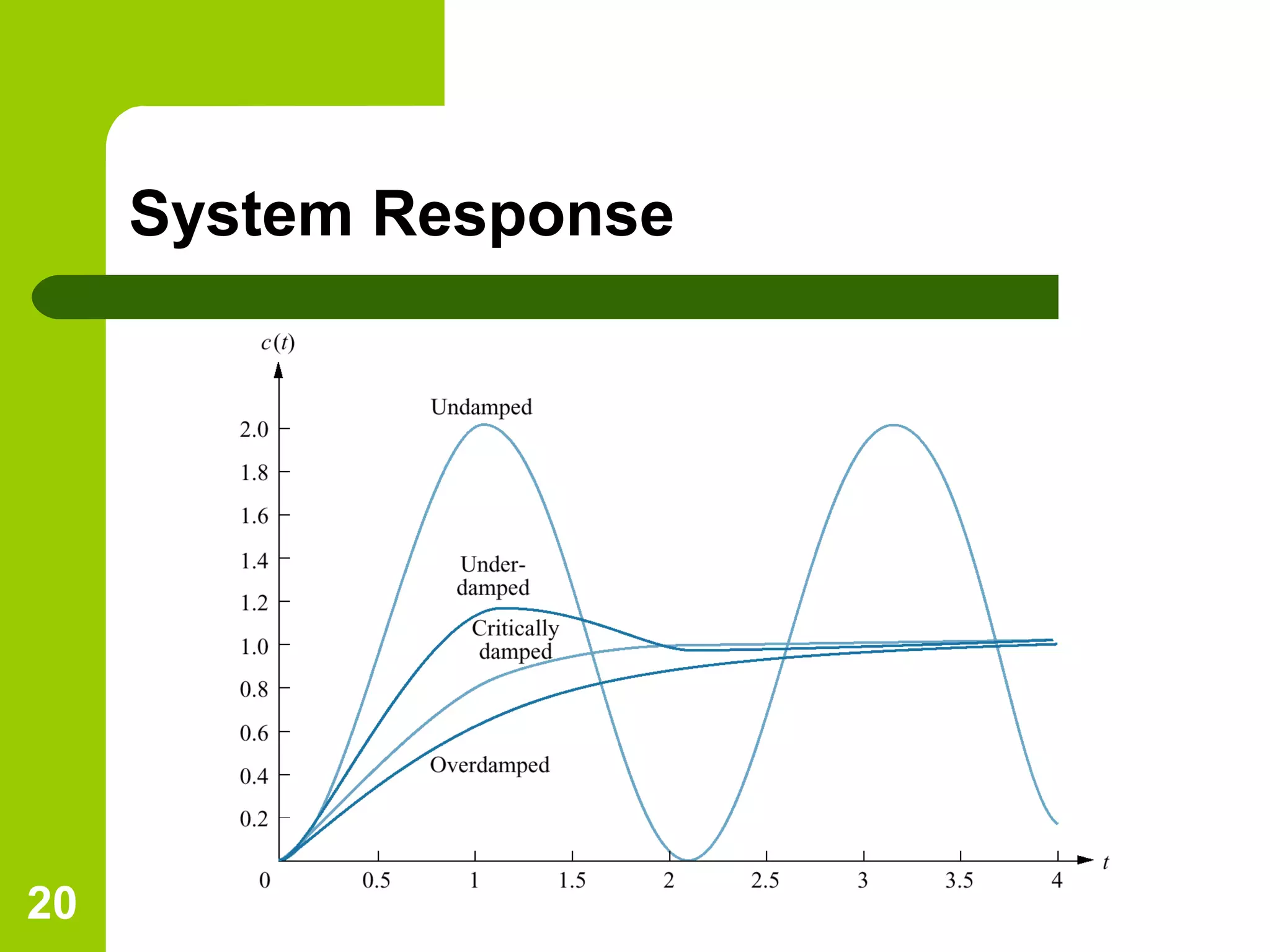
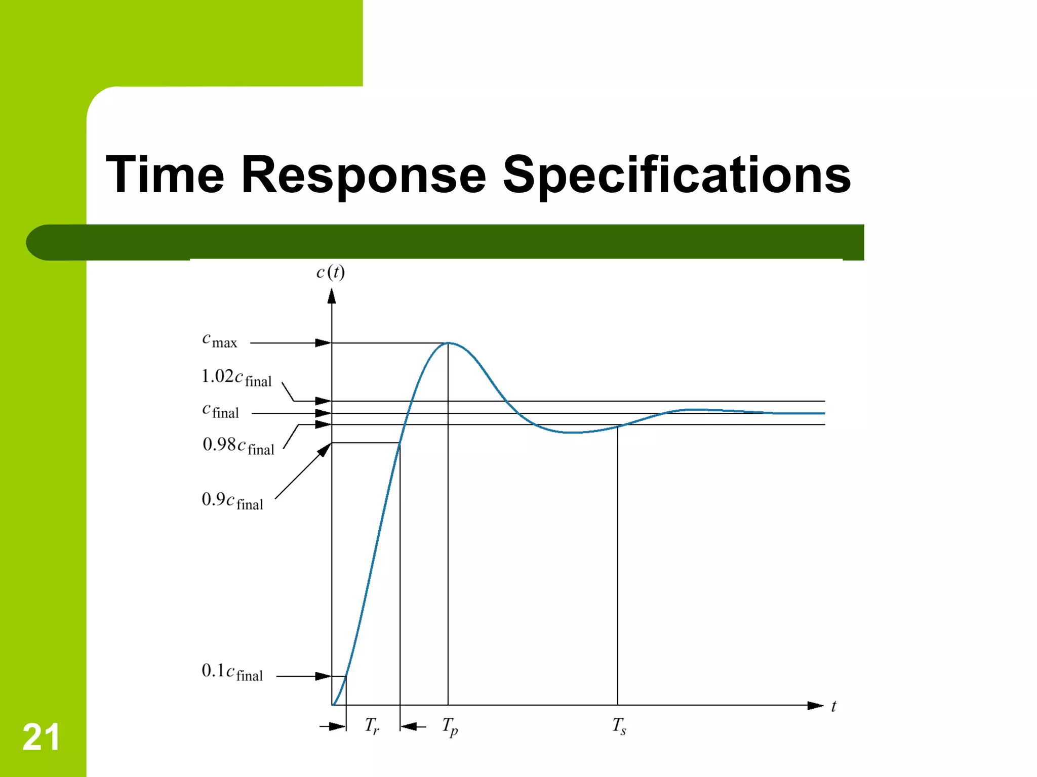
1. TIME RESPONSE ANALYSIS
SUBMITTED TO: SUBMITTED BY:
Somesh Chaturvedi Hariom (10655)
Asst. Proff. EE dept. B.tech (ME)
Career Point university 6TH
SEM.
TOPIC
Simulation between the transient part and steady
state part of the time response in terms of time
constant.

2. 2
Time Response Analysis
– Time Response
– Transient Response
– Steady state response
– Standard input signals
– First order system response
– Second order system response
– Time response analysis

3. 3
Time-Response Analysis
 Since time is used as an independent variable
in most control systems, it is usually of interest
to evaluate the state and the output responses
with respect to time or simply, the Time-
Response.
 In control system design analysis, a reference
input signal is applied to a system and the
performance of the system is evaluated by
studying the system response in the time-
domain.

4. 4
Time-Response
 The time-response of a control system is usually
divided into two parts namely; the Steady-
State Response and the Transient Response.
 In other words, the output response of a system
is the sum of two responses: the forced
response (steady-state response) and the
natural response (zero-input response).

5. 5
Time-Response of an Elevator

6. 6
Transient Response
 Defined as the part of the time response that
goes to zero as time goes to infinity.
 It does mot depend on input signal
 It gives information about the nature of
response and also give indication about
speed.

7. 7
Steady-State Response
 Defined as the part of the total response that
remains after the transient has died out.
 It depends on input signal.
 It gives the information about the accuracy of
the system.

8. 8
Standard Input Signals
 There are a number of standard inputs that are
considered simple enough and universal
enough that they are considered when
designing a control system.
 These inputs are known as a unit step, a ramp,
and a parabolic input functions.

9. 9
Unit Step Function
 A unit step function is defined piecewise as
such:
 The unit step function is a highly important
function, not only in control systems
engineering, but also in signal processing,
systems analysis, and all branches of
engineering.

10. 10
Unit Step Function

11. 11
Ramp Input Function
 A unit ramp is defined in terms of the unit step
function, as such: r(t) = tu(t).
 It is important to note that the ramp function is
simply the integral of the unit step function:

12. 12
Ramp Input Function

13. 13
Parabolic Input Function
 A unit parabolic input is similar to a ramp
input:
 Notice also that, the unit parabolic input is
equal to the integral of the ramp function:

14. 14
Parabolic Input Function

15. 15
First-Order Systems

16. 16
Initial Conditions are zero

17. 17
First-Order Systems Response

18. 18
System Response
K (1 − e−t /τ )
System response. K = gain
Response to initial condition

19. 19
Second-Order Systems Response
ζ = 0

20. 20
System Response

21. 21
Time Response Specifications

22. 22
Rise Time
 Is the amount of time that it takes for the system
response to reach the target value from an
initial state of zero.
 Rise time is defined as the time for the
waveform to go from 0.1 to 0.9 of its final value.
 Rise time is typically denoted tr, or trise.
 This is because some systems never rise to
100% of the expected, target value and
therefore, they would have an infinite rise-time.

23. 23
Settling Time
 After the initial rise time of the system, some systems
will oscillate and vibrate for an amount of time before
the system output settles on the final value.
 The amount of time it takes to reach steady state after
the initial rise time is known as the settling time
 Which is defined as the time for the response to reach
and stay within, 2% (or 5%) of its final value.
 Damped oscillating systems may never settle
completely.

24. 24
Settling time
nn
st
ζωζω
ζ 4102.0ln( 2
≈
−−
=⇒

25. 25
Peak Time
 The time required to
reach the first or
maximum peak. 2
1 ζω
π
−
=
n
pt
22
2
2
)()]([
nn
n
ss
ssCtcL
ωζω
ω
++
==
)1()(
1
1
222
2
2
ζωζω
ζω
ζ
ω
−++
−
−
=
nn
n
n
s

26. 26
Percent Overshoot
 The amount that the
waveform overshoots
the steady-state or final
value at the peak time,
expressed as a
percentage of the
steady-state value.
100%
max
×
−
=
final
final
c
cc
OS