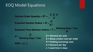
The document discusses the economic order quantity (EOQ) model, which aims to determine the optimal order quantity that minimizes total inventory costs. It defines key terms like inventory, setup costs, holding costs. The derivation of the EOQ formula is shown, which balances setup and holding costs to find the quantity that minimizes total annual costs. An example application for a company calculating optimal order quantity and reorder point is provided.

1. THE EOQ MODEL
HASNAIN BABER
ASSISTANT PROFESSOR
1

2. SOME BASIC DEFINITIONS
 An INVENTORY is an accumulation of a commodity that will be used to
satisfy some future demand.
 Inventories may be of the following form:
- Raw material
- Components (subassemblies)
- Work-in-process
- Finished goods
- Spare parts
2

3. 3EOQ History
• Introduced in 1913 by Ford W. Harris, “How Many Parts to Make at Once”
• Interest on capital tied up in wages, material and overhead sets a maximum
limit to the quantity of parts which can be profitably manufactured at one
time; “set-up” costs on the job fix the minimum. Experience has shown one
manager a way to determine the economical size of lots.
• Early application of mathematical modeling to Scientific Management

4. EOQ MODELING ASSUMPTIONS
1. Production is instantaneous – there is no capacity constraint and the entire lot is
produced simultaneously.
2. Delivery is immediate – there is no time lag between production and availability to
satisfy demand.
3. Demand is deterministic – there is no uncertainty about the quantity or timing of
demand.
4. Demand is constant over time – in fact, it can be represented as a straight line, so that
if annual demand is 365 units this translates into a daily demand of one unit.
5. A production run incurs a fixed setup cost – regardless of the size of the lot or the
status of the factory, the setup cost is constant.
6. Products can be analyzed singly – either there is only a single product or conditions
exist that ensure separability of products.
4

5. 5

6. 6

7. 7

8. 8
T
Q
Time
Inventory
MAX
Reorder
MIN
Buffer stock
Safety stock

9. EOQ Model
Order Quantity
Annual Cost

10. Order Quantity
Annual Cost
Holding Cost
EOQ Model

11. Why Order Cost Decreases
 Cost is spread over more units
Example: You need 1000 microwave ovens
Purchase Order
Description Qty.
Microwave 1000
Purchase Order
Description Qty.
Microwave 1
Purchase Order
Description Qty.
Microwave 1
Purchase Order
Description Qty.
Microwave 1
Purchase Order
Description Qty.
Microwave 1
1 Order (Postage $ 0.35) 1000 Orders (Postage $350)
Order
quantity

12. Order Quantity
Annual Cost
Holding Cost
Order (Setup) Cost
EOQ Model

13. Order Quantity
Annual Cost
Holding Cost
Total Cost Curve
Order (Setup) Cost
EOQ Model

14. Order Quantity
Annual Cost
Holding Cost
Total Cost Curve
Order (Setup) Cost
Optimal
Order Quantity (Q*)
EOQ Model

15. 15
• Holding cost per unit time =
 
2
levelinventoryAverage
Q
hh 

16. THE AVERAGE ANNUAL COST CURVE 16
unit time
cost
Q
2
hQ
G(Q)
Q
DS *
Q*
Annual fixed ordering
and holding cost
The minimum

17. EOQ Formula Derivation
D = Annual demand (units)
C = Cost per unit ($)
Q = Order quantity (units)
S = Cost per order ($)
I = Holding cost (%)
H = Holding cost ($) = I x C
Number of Orders = D / Q
Ordering costs = S x (D / Q)
Average inventory
units = Q / 2
$ = (Q / 2) x C
Cost to carry
average inventory = (Q / 2) x I x C
= (Q /2) x H
Total cost = (Q/2) x I x C + S x (D/Q)
inv carry cost order cost
Take the 1st derivative:
d(TC)/d(Q) = (I x C) / 2 - (D x S) / Q²
To optimize: set d(TC)/d(Q) = 0
DS/ Q² = IC / 2
Q²/DS = 2 / IC
Q²= (DS x 2 )/ IC
Q = sqrt (2DS / IC)

18. D = Annual demand (units)
S = Cost per order ($)
C = Cost per unit ($)
I = Holding cost (%)
H = Holding cost ($) = I x C
Economic Order Quantity
H
SD
EOQ


2

19. EOQ Model Equations
Optimal Order Quantity
Expected Number Orders
Expected Time Between Orders
Working Days / Year
Working Days / Year
 
 
 
 

 
Q
D S
H
N
D
Q
T
N
d
D
ROP d L
*
*
2
D = Demand per year
S = Setup (order) cost per order
H = Holding (carrying) cost
d = Demand per day
L = Lead time in days

20. EOQ
Example
You’re a buyer for SaveMart.
SaveMart needs 1000 coffee makers per year.
The cost of each coffee maker is $78.
Ordering cost is $100 per order. Carrying cost
is 40% of per unit cost. Lead time is 5 days.
SaveMart is open 365 days/yr.
What is the optimal order quantity & ROP?

21. SaveMart EOQ
H
SD
EOQ


2
20.31$
100$10002 
EOQ
D = 1000
S = $100
C = $ 78
I = 40%
H = C x I
H = $31.20
EOQ = 80 coffeemakers

22. SaveMart ROP
ROP = demand over lead time
= daily demand x lead time (days)
= d x l
D = annual demand = 1000
Days / year = 365
Daily demand = 1000 / 365 = 2.74
Lead time = 5 days
ROP = 2.74 x 5 = 13.7 => 14

23. Avg. CS = OQ / 2
= 80 / 2 = 40 coffeemakers
= 40 x $78 = $3,120
Inv. CC = $3,120 x 40% = $1,248
Note: unrelated to reorder point
SaveMart
Average (Cycle Stock) Inventory