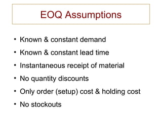
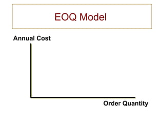
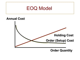
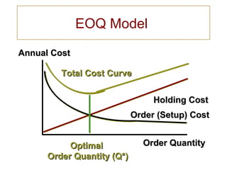
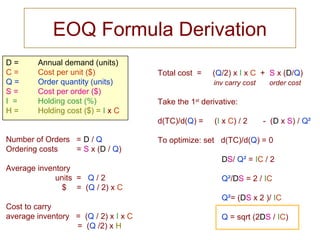
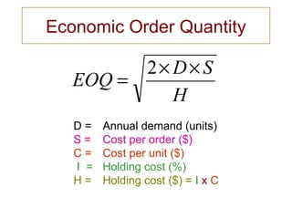
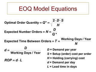
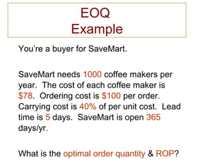
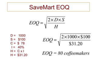
EOQ Model
Economic Order Quantity
Ken Homa
EOQ Assumptions
• Known & constant demand
• Known & constant lead time
• Instantaneous receipt of material
• No quantity discounts
• Only order (setup) cost & holding cost
• No stockouts
Inventory Holding Costs
Reasonably Typical Profile
Housing (building) cost 6%
Material handling costs 3%
Labor cost 3%
Inventory investment costs 11%
Pilferage, scrap, & obsolescence 3%
Total holding costTotal holding cost 26%26%
% of% of
CategoryCategory Inventory ValueInventory Value
EOQ Model
Order Quantity
Annual Cost
Order QuantityOrder Quantity
Annual CostAnnual Cost
Holding CostHolding Cost
EOQ Model
Why Order Cost Decreases
• Cost is spread over more units
Example: You need 1000 microwave ovens
Purchase Order
Description Qty.
Microwave 1000
Purchase Order
Description Qty.
Microwave 1
Purchase Order
Description Qty.
Microwave 1
Purchase Order
Description Qty.
Microwave 1
Purchase Order
Description Qty.
Microwave 1
1 Order (Postage $ 0.35)1 Order (Postage $ 0.35) 1000 Orders (Postage $350)1000 Orders (Postage $350)
OrderOrder
quantityquantity
Order QuantityOrder Quantity
Annual CostAnnual Cost
Holding CostHolding Cost
Order (Setup) CostOrder (Setup) Cost
EOQ Model
Order QuantityOrder Quantity
Annual CostAnnual Cost
Holding CostHolding Cost
Total Cost CurveTotal Cost Curve
Order (Setup) CostOrder (Setup) Cost
EOQ Model
Order QuantityOrder Quantity
Annual CostAnnual Cost
Holding CostHolding Cost
Total Cost CurveTotal Cost Curve
Order (Setup) CostOrder (Setup) Cost
OptimalOptimal
Order Quantity (Q*)Order Quantity (Q*)
EOQ Model
EOQ Formula Derivation
D = Annual demand (units)
C = Cost per unit ($)
Q = Order quantity (units)
S = Cost per order ($)
I = Holding cost (%)
H = Holding cost ($) = I x C
Number of Orders = D / Q
Ordering costs = S x (D / Q)
Average inventory
units = Q / 2
$ = (Q / 2) x C
Cost to carry
average inventory = (Q / 2) x I x C
= (Q /2) x H
Total cost = (Q/2) x I x C + S x (D/Q)
inv carry cost order cost
Take the 1st
derivative:
d(TC)/d(Q) = (I x C) / 2 - (D x S) / Q²
To optimize: set d(TC)/d(Q) = 0
DS/ Q² = IC / 2
Q²/DS = 2 / IC
Q²= (DS x 2 )/ IC
Q = sqrt (2DS / IC)
H
SD
EOQ
××
=
2
D = Annual demand (units)
S = Cost per order ($)
C = Cost per unit ($)
I = Holding cost (%)
H = Holding cost ($) = I x C
Economic Order Quantity
EOQ Model Equations
Optimal Order Quantity
Expected Number Orders
Expected Time Between Orders
Working Days / Year
Working Days / Year
= =
⋅ ⋅
= =
= =
=
= ⋅
Q
D S
H
N
D
Q
T
N
d
D
ROP d L
*
*
2
D = Demand per year
S = Setup (order) cost per order
H = Holding (carrying) cost
d = Demand per day
L = Lead time in days
EOQ
Example
You’re a buyer for SaveMart.
SaveMart needs 1000 coffee makers per
year. The cost of each coffee maker is
$78. Ordering cost is $100 per order.
Carrying cost is 40% of per unit cost. Lead
time is 5 days. SaveMart is open 365
days/yr.
What is the optimal order quantity & ROP?
SaveMart EOQ
H
SD
EOQ
××
=
2
20.31$
100$10002 ××
=EOQ
D = 1000
S = $100
C = $ 78
I = 40%
H = C x I
H = $31.20 EOQ = 80 coffeemakers
SaveMart ROP
ROP = demand over lead time
= daily demand x lead time (days)
= d x l
D = annual demand = 1000
Days / year = 365
Daily demand = 1000 / 365 = 2.74
Lead time = 5 days
ROP = 2.74 x 5 = 13.7 => 14
Avg. CS = OQ / 2
= 80 / 2 = 40 coffeemakers
= 40 x $78 = $3,120
Inv. CC = $3,120 x 40% = $1,248
Note: unrelated to reorder point
SaveMart
Average (Cycle Stock) Inventory
H
SD
EOQ
××
=
2
D = Annual demand (units)
S = Cost per order ($)
C = Cost per unit ($)
I = Holding cost (%)
H = Holding cost ($) = I x C
Economic Order Quantity
What if …
1. Interest rates go up ?
2. Order processing is automated ?
3. Warehouse costs drop ?
4. Competitive product is introduced ?
5. Product is cost-reduced ?
6. Lead time gets longer ?
7. Minimum order quantity imposed ?
H
SD
EOQ
××
=
2

ECONOMIC ORDER QTY

  • 1.
    EOQ Model Economic OrderQuantity Ken Homa
  • 2.
    EOQ Assumptions • Known& constant demand • Known & constant lead time • Instantaneous receipt of material • No quantity discounts • Only order (setup) cost & holding cost • No stockouts
  • 3.
    Inventory Holding Costs ReasonablyTypical Profile Housing (building) cost 6% Material handling costs 3% Labor cost 3% Inventory investment costs 11% Pilferage, scrap, & obsolescence 3% Total holding costTotal holding cost 26%26% % of% of CategoryCategory Inventory ValueInventory Value
  • 4.
  • 5.
    Order QuantityOrder Quantity AnnualCostAnnual Cost Holding CostHolding Cost EOQ Model
  • 6.
    Why Order CostDecreases • Cost is spread over more units Example: You need 1000 microwave ovens Purchase Order Description Qty. Microwave 1000 Purchase Order Description Qty. Microwave 1 Purchase Order Description Qty. Microwave 1 Purchase Order Description Qty. Microwave 1 Purchase Order Description Qty. Microwave 1 1 Order (Postage $ 0.35)1 Order (Postage $ 0.35) 1000 Orders (Postage $350)1000 Orders (Postage $350) OrderOrder quantityquantity
  • 7.
    Order QuantityOrder Quantity AnnualCostAnnual Cost Holding CostHolding Cost Order (Setup) CostOrder (Setup) Cost EOQ Model
  • 8.
    Order QuantityOrder Quantity AnnualCostAnnual Cost Holding CostHolding Cost Total Cost CurveTotal Cost Curve Order (Setup) CostOrder (Setup) Cost EOQ Model
  • 9.
    Order QuantityOrder Quantity AnnualCostAnnual Cost Holding CostHolding Cost Total Cost CurveTotal Cost Curve Order (Setup) CostOrder (Setup) Cost OptimalOptimal Order Quantity (Q*)Order Quantity (Q*) EOQ Model
  • 10.
    EOQ Formula Derivation D= Annual demand (units) C = Cost per unit ($) Q = Order quantity (units) S = Cost per order ($) I = Holding cost (%) H = Holding cost ($) = I x C Number of Orders = D / Q Ordering costs = S x (D / Q) Average inventory units = Q / 2 $ = (Q / 2) x C Cost to carry average inventory = (Q / 2) x I x C = (Q /2) x H Total cost = (Q/2) x I x C + S x (D/Q) inv carry cost order cost Take the 1st derivative: d(TC)/d(Q) = (I x C) / 2 - (D x S) / Q² To optimize: set d(TC)/d(Q) = 0 DS/ Q² = IC / 2 Q²/DS = 2 / IC Q²= (DS x 2 )/ IC Q = sqrt (2DS / IC)
  • 11.
    H SD EOQ ×× = 2 D = Annualdemand (units) S = Cost per order ($) C = Cost per unit ($) I = Holding cost (%) H = Holding cost ($) = I x C Economic Order Quantity
  • 12.
    EOQ Model Equations OptimalOrder Quantity Expected Number Orders Expected Time Between Orders Working Days / Year Working Days / Year = = ⋅ ⋅ = = = = = = ⋅ Q D S H N D Q T N d D ROP d L * * 2 D = Demand per year S = Setup (order) cost per order H = Holding (carrying) cost d = Demand per day L = Lead time in days
  • 13.
    EOQ Example You’re a buyerfor SaveMart. SaveMart needs 1000 coffee makers per year. The cost of each coffee maker is $78. Ordering cost is $100 per order. Carrying cost is 40% of per unit cost. Lead time is 5 days. SaveMart is open 365 days/yr. What is the optimal order quantity & ROP?
  • 14.
    SaveMart EOQ H SD EOQ ×× = 2 20.31$ 100$10002 ×× =EOQ D= 1000 S = $100 C = $ 78 I = 40% H = C x I H = $31.20 EOQ = 80 coffeemakers
  • 15.
    SaveMart ROP ROP =demand over lead time = daily demand x lead time (days) = d x l D = annual demand = 1000 Days / year = 365 Daily demand = 1000 / 365 = 2.74 Lead time = 5 days ROP = 2.74 x 5 = 13.7 => 14
  • 16.
    Avg. CS =OQ / 2 = 80 / 2 = 40 coffeemakers = 40 x $78 = $3,120 Inv. CC = $3,120 x 40% = $1,248 Note: unrelated to reorder point SaveMart Average (Cycle Stock) Inventory
  • 17.
    H SD EOQ ×× = 2 D = Annualdemand (units) S = Cost per order ($) C = Cost per unit ($) I = Holding cost (%) H = Holding cost ($) = I x C Economic Order Quantity
  • 18.
    What if … 1.Interest rates go up ? 2. Order processing is automated ? 3. Warehouse costs drop ? 4. Competitive product is introduced ? 5. Product is cost-reduced ? 6. Lead time gets longer ? 7. Minimum order quantity imposed ? H SD EOQ ×× = 2