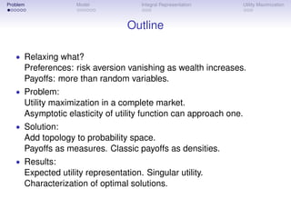
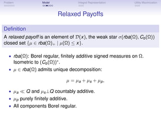
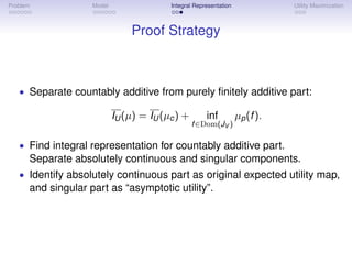
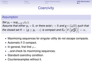
This document provides an outline and summary of a presentation on relaxing the assumptions of utility maximization in complete markets. It discusses relaxing preferences to allow risk aversion to decline to zero as wealth increases, and relaxing payoffs to include more than just random variables. The presentation introduces a model that uses measures instead of densities to represent payoffs, and relaxes the utility functional. It presents results on an expected utility representation involving both absolutely continuous and singular components, and characterizes optimal solutions. The document provides context and motivation for considering cases where the asymptotic elasticity of the utility function approaches one.

1. Problem Model Integral Representation Utility Maximization
Relaxed Utility Maximization
in Complete Markets
Paolo Guasoni
(Joint work with Sara Biagini)
Boston University and Dublin City University
Analysis, Stochastics, and Applications
In Honor of Walter Schachermayer
July 15th , 2010

2. Problem Model Integral Representation Utility Maximization
Outline
• Relaxing what?
Preferences: risk aversion vanishing as wealth increases.
Payoffs: more than random variables.
• Problem:
Utility maximization in a complete market.
Asymptotic elasticity of utility function can approach one.
• Solution:
Add topology to probability space.
Payoffs as measures. Classic payoffs as densities.
• Results:
Expected utility representation. Singular utility.
Characterization of optimal solutions.

3. Problem Model Integral Representation Utility Maximization
The Usual Argument
• Utility Maximization from terminal wealth:
max{EP [U(X )] : EQ [X ] ≤ x}
• Use first-order condition to look for solution:
ˆ dQ
U (X ) = y
dP
• Pick the Lagrange multiplier y which saturates constraint:
ˆ
EQ X (y ) = x
• If there is any.
• Assumptions on U?

4. Problem Model Integral Representation Utility Maximization
The Usual Conditions
• Karatzas, Lehoczky, Shreve, and Xu (1991):
U (βx) < αU (x) for all x > x0 > 0 and some α < 1 < β
• This condition implies the next one.
• Kramkov and Schachemayer (1999):
xU (x)
AE(U) = lim sup <1
x↑∞ U(x)
• Guarantees an optimal payoff in any market model.
• Condition not satisfied? No solution for some model.
• Interpretation?

5. Problem Model Integral Representation Utility Maximization
Asymptotic Relative Risk Aversion
• What do these conditions mean (and imply)?
• Suppose Relative Risk Aversion has a limit:
xU (x)
ARRA(U) = lim −
x↑∞ U (x)
• Then AE(U) < 1 is equivalent to ARRA(U) > 0.
• As wealth increases, risk aversion must remain above ε > 0.
• Why? Lower risk premium when you are rich?
• AE(U) = 1 as Asymptotic Relative Risk Neutrality.
• Relative Risk Aversion positive. But declines to zero.
• “Relaxed” Investor.
• Relevance?

6. Problem Model Integral Representation Utility Maximization
Who Cares?
• Logarithmic, Power, and Exponential utilities satisfy ARRA(U) > 0.
• Why bother about ARRA(U) = 0, if there are no examples?
• Heterogeneous preferences equilibria.
Benninga and Mayshar (2000), Cvitanic and Malamud (2008).
• Complete market with several power utility agents.
Power of utility depends on agent.
• Utility function of representative agent.
Relative risk aversion decreases to that of least risk averse agent.
• All values of relative risk aversion present in the market?
Risk aversion of representative agent decreases to zero.
• Asymptotic elasticty equals one. Solution may not exist.
• But why?

7. Problem Model Integral Representation Utility Maximization
Singular Investment
• Kramkov and Schachermayer (1999) show what goes wrong.
• Countable space Ω = (ωn )n≥1 . dP/dQ(ωn ) = pn /qn ↑ ∞ as n ↑ ∞.
• Finite space ΩN . ωn = ωn for n < N. (ωn )n≥N lumped into ωN .
N N
• Solution exists in each ΩN . Satisfies first order condition:
N N
U (Xn ) = y qn /pn 1≤n<N U (XN ) = y qN /pN
N N−1 N N−1
where pN = 1 − n=1 pn and qN = 1 − n=1 qn .
• What happens to N
(Xn )1≤n≤N as N ↑ ∞?
N
• Xn → Xn , which solves U (Xn ) = yqn /pn for n ≥ 1.
• For large initial wealth x, EQ [X ] < x. Where has x − EQ [X ] gone?
N N N
• qN XN converges to x − EQ [X ]. But qN decreases to 0.
• Invest x − EQ [X ] in a “payoff” equal to ∞ with 0 probability.

8. Problem Model Integral Representation Utility Maximization
Main Idea
• The problem wants to concentrate money on null sets.
• But expected utility does not see such sets.
• Relax the notion of payoff.
• Relax utility functional.
• Do it consistently.

9. Problem Model Integral Representation Utility Maximization
Setting
• (Ω, T ) Polish space.
• P, Q Borel-regular probabilities on Borel σ-field F.
• Q∼P
• Payoffs available with initial capital x: C(x) := {X ∈ L0 |EQ [X ] ≤ x}
+
• Market complete.
• U : (0, +∞) → (−∞, +∞)
strictly increasing, strictly concave, continuously differentiable.
• Inada conditions U (0+ ) = +∞ and U (+∞) = 0.
• supX ∈C(x) EP [U(X )] < U(∞)
• P (and hence Q) has full support, i.e. P(G) > 0 for any open set G.
• If not, replace Ω with support of P.

10. Problem Model Integral Representation Utility Maximization
Relaxed Payoffs
Definition
A relaxed payoff is an element of D(x), the weak star σ(rba(Ω), Cb (Ω))
closed set {µ ∈ rba(Ω)+ | µ(Ω) ≤ x}.
• rba(Ω): Borel regular, finitely additive signed measures on Ω.
Isometric to (Cb (Ω))∗ .
• µ ∈ rba(Ω) admits unique decomposition:
µ = µ a + µs + µp ,
• µa Q and µs ⊥Q countably additive.
• µp purely finitely additive.
• All components Borel regular.

11. Problem Model Integral Representation Utility Maximization
Finitely Additive?
• Dubious interpretation of finitely additive measures as payoffs.
• Allow them a priori. For technical convenience.
• Let the problem rule them out.
• They are not optimal anyway.

12. Problem Model Integral Representation Utility Maximization
Relaxed Utility
• Relaxed utility map IU : rba(Ω) → [−∞, +∞).
• Defined on rba(Ω) as upper semicontinuous envelope of IU :
IU (µ) = inf{G(µ) | G weak ∗ u.s.c., G ≥ IU on L1 (Q)}.
• Relaxed utility maximization problem:
max IU (µ)
µ∈D(x)
• Relaxed utility map IU weak star upper semicontinuous.
• Space of relaxed payoffs D(x) weak star compact.
• Relaxed utility maximization has solution by construction.
• Elaborate tautology.
• Find “concrete” formula for IU . Integral representation.

13. Problem Model Integral Representation Utility Maximization
Singular Utility
• V (y ) = supx>0 (U(x) − xy ) convex conjugate of U.
• Singular utility: nonnegative function ϕ defined as:
dQ
ϕ(ω) = inf g(ω) g ∈ Cb (Ω), EP V g <∞ ,
dP
• Upper semi-continuous, as infimum of continuous functions.
• Defined for all ω. Function, not random variable.
• W : Ω × R+ → R sup-convolution of U and x → xϕ(ω) dQ (ω):
dP
dQ
W (ω, x) := sup U(z) + (x − z)ϕ(ω) (ω) .
z≤x dP
• ϕ(ω) = 0 for each ω where dP/dQ is bounded in a neighborhood.
• Concentrating wealth suboptimal if odds finite.
• ϕ may be positive only on poles of dP/dQ.

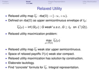
14. Problem Model Integral Representation Utility Maximization
Integral Representation
Theorem
Let µ ∈ rba(Ω)+ , and Q ∼ P fully supported probabilities.
i) In general:
dµa
IU (µ) = EP W ·, + ϕdµs + inf µp (f ).
dQ f ∈Cb (Ω),EP [V (f dQ )]<∞
dP
ii) If ϕ = 0 P-a.s., then:
dµa
IU (µ) = EP U + ϕdµs + inf µp (f ).
dQ f ∈Cb (Ω),EP [V (f dQ )]<∞
dP
xU (x)
iii) If lim supx↑∞ U(x) < 1, then {ϕ = 0} = Ω and
dµa
IU (µ) = EP U .
dQ

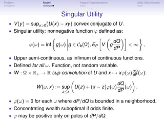
15. Problem Model Integral Representation Utility Maximization
Three Parts
• First formula holds for any µ ∈ rba(Ω)+ .
• But has finitely additive part...
• ...and has sup-convolution W instead of U.
• Second formula replaces W with U under additional assumption.
• Then utility is sum of three pieces.
• Usual expected utility E[U(X )] with X = dµa .
dQ
• Finitely additive part.
• Singular utility ϕdµs .
• Accounts for utility from concentration of wealth on P-null sets.
• ϕ(ω) represents maximal utility from Dirac delta on ω
• Only usual utility remains for AE(U) < 1.

16. Problem Model Integral Representation Utility Maximization
Proof Strategy
• Separate countably additive from purely finitely additive part:
IU (µ) = IU (µc ) + inf µp (f ).
f∈ Dom(JV )
• Find integral representation for countably additive part.
Separate absolutely continuous and singular components.
• Identify absolutely continuous part as original expected utility map,
and singular part as “asymptotic utility”.

17. Problem Model Integral Representation Utility Maximization
Coercivity
Assumption
Set y0 = supω∈Ω ϕ(ω).
Assume that either y0 = 0, or there exist ε > 0 and g ∈ Cb (Ω) such that
the closed set K = {g ≥ y0 − ε} is compact and EP V g dQ < ∞.
dP
• Maximizing sequences for singular utility do not escape compacts.
• Automatic if Ω compact.
• In general, first find ϕ...
• ...and check its maximizing sequences.
• Standard coercitivy condition.
• Counterexamples without it.

18. Problem Model Integral Representation Utility Maximization
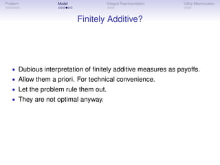
Relaxed utility Maximization
Theorem
Under coercivity assumption, and if ϕ = 0 a.s.:
i) u(x) = maxµ∈D(x) IU (µ);
dµ∗
ii) u(x) = E[U(X ∗ (x))] + ϕdµ∗ , where X ∗ (x) =
s dQ .
a
iii) Budget constraint binding: µ∗ (Ω) = EQ [X ∗ (x)] + µ∗ (Ω)
s = x.
iv) µ∗ unique. Support of any µ∗ satisfies:
a s
supp(µ∗ ) ⊆ argmax(ϕ).
s
v) If x > x0 , any solution has the form µ∗ = µ∗ + µ∗ , where
a s
µ∗ (Ω) = x − x0 .
s
vi) u(x) = u(x0 ) + (x − x0 ) maxω ϕ(ω) = u(x0 ) + (x − x0 )y0 .

19. Problem Model Integral Representation Utility Maximization
Conclusion
Happy Birthday for your first 60!
Ad Maiora et Meliora!