The document discusses key concepts in probability theory critical for predictive analytics, including important terminologies, theorems, and special probability distributions. It emphasizes that understanding probability can enhance predictions in data analytics projects, especially when dealing with big data. The chapter further explains various types of random variables, distribution functions, and conditional probabilities, providing illustrations and application scenarios.

1. PROBABILITY FOR DATA ANALYTICS
Dr.S.Saudia,
Assistant Professor,
CITE, M.S.University

2. Objectives of the Chapter.
• To understand different Probability concepts for application in
different Predictive Analytics.
• To understand different hypothesis testing procedures .

3. Chapter contents.
1. Important Terminologies in Probability Theory: Random Experiment,
Outcome, Event, Mutually exclusive event, Exhaustive event, Equally likely
event.
2. Probability: definitions, theorems of Probability, Conditional Probability,
Random Variable, Discrete Probability distribution, Cumulative Distribution
Function, Joint Distribution of two variables.
3. Some special probability distribution: Binomial, Poison, Geometric,
Uniform, Normal. Multivariate normal distribution - Sampling distribution .

4. Importance of Probability Theory
So in Data analytics projects, you have that BIG DATA and you need to make best
prediction for the associated industry/ organization/ Sector in the predictive Analytics stage of the Data Analytics
Project.
The best predictions can be made with a knowledge on the concepts of Probability Theory.
It is a mathematical theory with concepts for modeling predictions of unpredictable events or phenomenon [1].
Should I stop Smoking? The probabilities on the risk of getting cancer & risk of
committing suicide made me continue [2]

5. Well! this’s another cartoon [3] which
I found while hunting for pics.
on Probabilty theory.
Ha .. Ha..
But don’t keep away from Probability theory.
It matters for Data Analytics and
Of Course for a reason to continue Smoking…..
Hee.. Hee..
Saudia

6. 1. Important Terminologies in Probability Theory[4]
•Random Experiment: Random experiments are experiments whose outcome cannot be predicted.
Eg: Finding the structure of next generation genes.
Finding the price of a Stock tomorrow.
Finding the risk of next generation getting diabetes.
•Outcome: The possible result of a random experiment is called an outcome. Outcomes cannot be split further.
Eg: In the experiment involving finding the structure of next generation genes, the total number of possible
outcomes shall be 2n combinations of the different n components of the genes.
•Event : One of the outcomes which has occurred for an experiment is called an event.
Composite events: Events that can be decomposed to simpler events.
Elementary events: If the experiment produces only one outcome, then it is called an elementary event.
Eg: The set of all possible prices for a stock-Outcome
The set prices posssible tomorrow and which draws profit- Event.
Random Experiment[4]

7. •Mutually exclusive event : Two events are said to be mutually exclusive if they cannot occur
simultaneously.
Eg: A student choosing a second language. It is like either Tamil or HIndi.
•Exhaustive set: Several events are said to form an exhaustive set, if one of them must necessarily occur. The
group of all possible elementary events constitute the Exhaustive set.
Eg: The set of all possible combination of genes for the next generation.
•Equally likely event: Two events are equally likely if the chances of their occurrence is equally likely or
otherwise none of them can be expected in preference to another.
Eg: If successive generations all look alike, then some dominant trait is playing its role. The events are not
equally likely then.
2. Probability [1]
Definition: If in a random experiment which has n possible outcomes which are mutually exclusive, exhaustive and
equally likely, and m of these are favorable to an event A, the probability of the event is defined as the ratio m/n.
( )
( )
number of outcomes which are favourable events
Total number of outcomes of the random experiment.
0 1
mP A
n
P A
P
=
=
≤ ≤

8. An illustration to Probability of some events [5]
Consider a situation where there are 8 green cubes, 9 green spheres, 5 yellow cubes
and 7 yellow spheres.
Now let us know the probability of getting different objects from the bag.
Probability of getting a cube from the bag = 13 cubes can be drawn out from 29 equally likely objects.
= 13 cubes / 29 objects.
Probability of getting an yellow object from the bag = 12 objects can be drawn out from 29 objects.
= 12 objects / 29 objects.
The intersection area corresponds to
Region having cubes which are
yellow in colour.

9. An illustration to Probability of some events [5] contd..
Probability of getting an yellow cube from the bag = 5 yellow cubes can be drawn out from 29 objects.
= 5 cubes / 29 objects.
This yellow cubes will be in the area of intersection shown below. This shaded area correspond to cubes which are
yellow in color.
Probability of getting an yellow object or a cube of any color= 12 yellow objects+8 cubes (13 cubes-5 yellow cubes)
that can be drawn out from 29 objects.
P(Yellow or Cube) =(12+8) objects / 29 objects.= 20/29 objects.
This can also be written as
=Probability of getting one of 12 yellow objects + Probability of getting one cube-
Probability of yellow cubes.
=P(Yellow)+P(Cube)-P(Yellow and Cube)
Thus,
P(A or B)= P(A)+ P(B) – P(A and B) [Here A and B are not mutually exclusive
or otherwise A and B overlap].
This is the Addition Theorem of probability for events that are not
Mutually Exclusive.
12 13 5
29 29 29
+ −

10. An illustration to Probability of some events [5] contd..
If A and B are mutually exclusive or if their spaces do not overlap as shown below,
P(A or B)= P(A)+ P(B). This is the Addition Theorem for events that are Mutually Exclusive.
Theorems of Probability:
1.Addition Theorem:
When A and B are mutually exclusive,
or
When A and B are not mutually exclusive,
2. Probability of Complementary event:
( ) ( ) ( )
( ) ( ) ( )
P A B P A P B
P A or B P A P B
∪ = +
= +
( )1P A P A
−
 
= − 
 
( ) ( ) ( ) ( )
( ) ( ) ( ) ( )
ANDP A B P A P B P A B
P AorB P A P B P AB
∪ = + −
= + −

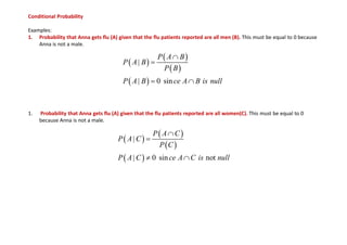
11. Conditional Probability
1.An illustration of Conditional Probability [6,7]
Consider a class of 100 students of whom 40 students opt to study maths, 30 students opt for biology and 20
students opt to study both biology and maths. What is the probability that a student who has taken maths will taken
biology?
The details are represented as a Venn diagram as shown below.
A is the group of students taking maths, B is the group of students taking biology.
Probability of a random student taking biology provided similarly,
that he has taken maths is given by
This is called Conditional Probability.
[In P(A|B, ‘|’ means ‘given that’)].
( )
( )
( )
( )
|
|
probability of A and B
P B A
probability of A
P A B
P B A
P A
=
∩
=
( )
( )
20 /100
|
40 /100
.2
| 0.5
.4
P B A
P B A
=
= =
( )
( )
( )
( )
|
|
probability of A and B
P A B
probability of B
P A B
P A B
P B
=
∩
=
( )
( )
20 /100
| B
30 /100
.2
| B 0.67
.3
P A
P A
=
= =

12. Theorems of Probability:
3.Multiplication Theorem:
When A and B are mutually exclusive,
or
When A and B are not mutually exclusive,
( ) ( ) ( )
( ) ( ) ( )
.
.
P A B P A P B
P A and B P A P B
∩ =
=
( ) ( ) ( ) ( ) ( )
( ) ( ) ( ) ( ) ( )
. | . |
. | . |
P A B P A P B A P B P A B
P A and B P A P B A P B P A B
∩ = =
= =

13. Conditional Probability
2.An illustration of Conditional Probability [6,7]
A represents taking bagel for breakfast, B represents taking pizza for lunch.
Given:
P(A) =0.6, P(B)=0.5,
P(A|B)=0.7
(The events A and B are dependent events since the probability of A and the probability of A when B has occurred are
different. )
Solution:
We know P(A and B)= P(B). P(A|B)=0.5x0.7=0.35
Also P(A and B)= P(A). P(B|A)
So P(B|A)= P(A and B)/ P(A) =0.35/ 0.6 =0.58

14. Conditional Probability
Examples:
1. Probability that Anna gets flu (A) given that the flu patients reported are all men (B). This must be equal to 0 because
Anna is not a male.
1. Probability that Anna gets flu (A) given that the flu patients reported are all women(C). This must be equal to 0
because Anna is not a male.
( )
( )
( )
( )
|
| 0 sin
P A B
P A B
P B
P A B ce A B is null
∩
=
= ∩
( )
( )
( )
( )
|
| 0 sin not
P A C
P A C
P C
P A C ce A C is null
∩
=
≠ ∩

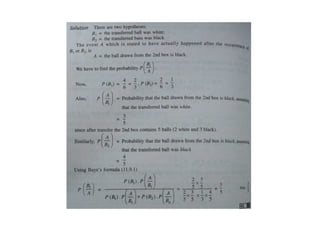
15. Bayes’ Theorem
Consider an event A which can occur if one of the mutually exclusive and exhaustive set of events B1, B2, B3,…
occurs.
If the unconditional probabilities, P(B1), P(B2) ,P(B3), P(B4),… and the conditional probabilities,
are known in prior, then the conditional probability of a specified event Bi, when A is said to have
occurred is given by the Bayes’ Theorem as given below.
Exercise:
Two boxes contain respectively 4 white and 2 black, and 1 white and 3 black balls. One ball is transferred from
the first box into the second, and then one drawn from the latter. It turns out to be black. What is the probability that the
transferred ball was white?
Solution: Refer Page 380 of [4].
1 2 3
, , ,...
A A A
P P P
B B B
    
    
     
( )
( )
1
i
ii
n
i
i i
A
P B P
BB
P
A A
P B P
B=
 
 
   = 
  
 
 
∑

17. Random Variable [4]:
Let S be the sample space of outcomes of some given random experiment. The outcomes of the experiments are not always
numbers. A function can be defined to assign a real number to each sample point. This function is called a Random
Variable or a Stochastic Variable.
Eg: In a random experiment of inheriting 2 genes A , B, the sample space is
A random variable, X can be defined on this Sample space as the ‘the number of A inherited’. Now a number can be
assigned to each sample point as:
If a Random Variable assumes a finite number of values, the Random Variable is a Discrete Random Variable.
In the above example, the random variable X takes only 3 values. So it is countable and so the random variable X is a
Discrete Random Variable.
If a Random Variable assumes a infinite number of values, the Random Variable is a Continuous Random Variable.
{ }, ,BA,BBS AA AB=
( ) 2, ( ) 1, ( ) 1, ( ) 0X AA X AB X BA X BB= = = =

18. Discrete Probability Distribution [4]:
Let X be a discrete random variable, x1,x2,x3,… be the possible values of X and p1,p2,p3,… be the probabilities
of those values.
Now the function, f which associates the values xi with their corresponding probabilities is called Discrete
Probability Distribution of X.
It satisfies two conditions:
Continuous Probability Distribution:
Let X be a continuous random variable, x1,x2,x3,… be the possible infinite number of values of X and
p1,p2,p3,… be the probabilities of those values.
Now the function, f which associates the values xi with their corresponding probabilities is called Continuous
Probability Distribution of X.
( ) ( )f x P X x= =
( )
( )
0
1
f x
f x
≥
=∑
It satisfies two conditions:
( )
( )
0
1
f x
f x dx
∞
−∞
≥
=∫

19. Cumulative Distribution Function (CPF) [4]:
Let X be a discrete random variable, x1,x2,x3,… be the possible values of X and p1,p2,p3,… be the probabilities
of those values.
Then the cumulative distribution function, F of a value x is the sum of probabilities of values of X which are less
than or equal to x.
It satisfies the condition:
For continuous probability distribution, f(x) of a continuous random variable, X in the interval , the cumulative
distribution function is given
( ) 1
1 1 2
1 2 2 3
1 2
0 when x<x
= p when x x<x
= p +p when x x<x
=p +p +...+p =1when x xn n
F x
and so on
=
≤
≤
≤
( )0 1F x≤ ≤
a x b≤ ≤
( ) ( )
b
a
F X f x dx= ∫

20. Joint Distribution of Two Variables [4]:
Let S be the sample space of a random experiment. We may assign two real numbers X(e) and Y(e) to each
sample point e of S according to some given rules.
X and Y are the two random variables of S. Now the possible pair of values for the variables, X and Y along with the
probabilities for all the pairs corresponds to the Joint Distribution or the Bivariate Distribution.
Illustration:
Four fair coins are tossed. If X and Y are
the random variables for ‘number of heads’ and the
‘longest run of heads’, construct the joint distribution
of X and Y.

21. Some special probability distribution [4]:
Probability Distribution of a random variable is the set of all possible values along with their probabilities.
Some theoretical distributions are: 1. Binomial 2. Poisson 3. Geometric, Normal.
Illustrations of some Discrete Probability Distribution:

22. If f(x) is known, pi is obtained by putting xi in the place of x as shown below.
Illustration
Here
Here f(x)=1/6

23. Expectation, Mean, Variance, Moments of a Random Variable
Let X be a discrete random variable, x1,x2,x3,…xn be the possible values of X and p1,p2,p3,…pn be the
probabilities of those values.
Then the Expectation or expected value of X- written as E(X) is defined as the sum of the products of its values and their
corresponding probabilities as shown below.
the Expectation or expected value of any function g(x)- is
Mean of a probability distribution is the expected value of X
Variance is the expected value of
The positive square root of variance gives standard deviation
Rth moment about A
( )
( )2 2
i i
i i
E X p x
E X p x
=
=
∑
∑
( )( ) ( )i iE g x p g x= ∑
, (X)Mean Eµ =
( )
2
x µ−
( )
2 2
2 2
, ( )Variance E x
is also equal to E x
σ µ
µ
= −
−
( )σ
'
( )r
r E x Aµ = −

24. Uniform Distribution (Discrete)
Let X be a discrete random variable, x1,x2,x3,…xn be the possible values of X and p1,p2,p3,…pn be all equal to a
constant 1/n.
The probability distribution defined by the probability mass function (p.m.f),
( ) ( )1 21/ ; , ,.... nf x n x x x x= =

25. Uniform Distribution (Continuous)
Let X be a continuous random variable. Then the Uniform distribution of this continuous variable is such that
probabilities associated with intervals of equal length are equal at any part of the range as shown in the figure below.
Where
a,b are the minimum possible and maximum possible values of X.
This distribution looks rectangular over .
This is also called Rectangular Distribution.
For a continuous random variable X, probability of the variable X is given by the area of the curve and it must be equal to
1.
Here, the curve is a rectangle and so the area = length x breadth
= (b-c) x f(x)
But area =1
So b-a x f(x)=1
Thus continuous uniform distribution is f(x)=1/ b-a
Uniform Distribution (Continuous) [8]
( ) 1/ b a;f x = −
a x b≤ ≤

28. Binomial Distribution (Discrete)
It is a discrete probability distribution for a random experiment where there are only two mutually exclusive
events and if the probability of success in each trial is a constant ‘p’ and the probability of failure is ‘q’ or (1-p), then in a
series of n trials, the probability of x successes is given by the below function, the Binomial probability distribution.
Here p+q=1 and
Example of random experiment whose probability of success is :0.5 [9]
Find f(x).
( ) x n x
xf x nC p q −
=
( )
!
! !
x
n
nC
x n x
=
−

29. Example:2 [9]
Find f(x).
2
,
,
Mean of binomial probability distribution np
Variance of binomial distribution npq
Standard deviationof binomial distribution npq
σ
σ
=
=
=

30. Exercises:
Investigate experiments whose events follow uniform and binomial distribution.

31. Poisson Distribution (Discrete)
It is a discrete probability distribution.
The probability of successful events is defined as
Here ‘m’ is the expected number of events per the time interval and is always positive. The x values ranges
from 0 to infinity.
Eg: It is mostly used to describe events which are occurring in a fixed time interval or region.
1. How many customers an ATM gets an hour?
2. How many vehicles pass through a signal in an hour?
Find f(x).
( )
.
!
m x
e m
f x
x
−
=
Poisson Distribution (Discrete) [10]

33. An Illustration

34. This can be found by determining the cdf of all probabilities of values

35. Number of clicks in an hour corresponds to the total number of clicks in a day (12) to the number of hours
in a day (24).
= 12/24
This is now the mean of the events.
So the probability of more than 1 click in the first hour is obtained as the cumulative density function of all the
probabilities of values greater than 1 with mean 0.5.
This can be found by determining the cdf of all probabilities of values greater than 1.

36. Normal Distribution (Gaussian Distribution )
It is an important continuous probability distribution which occur commonly. The probability density function is
given by
Here is the mean and is the standard deviation.
Eg:1
Normal Distribution of the heights of a population. [11]
( )
( )
( )
2
2
2
1
;
2
x
f x e x
x
µ
σ
σ
−
−
= −∞ < < ∞
µ σ

37. For standard normal distribution/ symmetric bell shaped population, the mean is 0 it is experimentally
determined that:
68% of the values lie within
95% of the values lie within
99.7% of the values lie within
Standard deviation fluctuates less when compared other measures of dispersion when moving from sample to
sample.
x σ
−
±
2x σ
−
±
3x σ
−
±
Normal Distribution of a population. [11]

38. Exercise:
Find the probability distribution functions of Exponential, Gamma, Erlang, Multivariate normal distribution
and understand their importance.
Sampling Distribution
Sampling Distribution of a statistic is the probability distribution of that statistic or otherwise the distribution
of the statistics of different samples of same size that are drawn repeatedly from the population.
Consider the situation of finding the average age of a class of 16 students. Let the population mean,
is to be found. This is done by finding the sample mean, of different samples of same size 3.
Let samples of size 3 be randomly selected and their sample mean values be equal to: 232.67, 255.
These sample mean is thus understood to vary from sample to sample as shown in the figure.
These sample means (16C3=560) of the population
when represented as a distribution it appears
normal about the sample mean mostly as shown
below as a histogram.
From this sampling distribution of sample means, statements can be
made on the population’s parameter values:
The parameter mean value which is the
mean of sample means.
Standard deviation of sample means from the true
mean is equal to the standard error of all sample means.
Standard error of sample mean =
Standard error of sample proportion, P =
µ x
−
Sample 1, Sample 2 [12]
Normal distribution of sample means. [12]
n
σ
PQ
n

39. References:
[1] www.google.com
[2] https://memeguy.com
[3] http://controlcartoons.com/
[4] Statistical methods, ‘N. G.Das’, McGraw Hill Companies.
[5] https://stats.stackexchange.com
[6] https://www.youtube.com
[7]www.youtube.com/watch?v=eHfhpAhGdvY
[8] https://www.youtube.com/watch?v=-qt8CPIadWQ
[9] http://study.com/academy/lesson/binomial-distribution
[10] https://www.youtube.com/watch?v =cPOChr_kuQs
[11] www.youtube.com/watch?v=iYiOVISWXS4
[12] https://www.youtube.com/watch?v=Zbw-YvELsaM
[13] https://www.youtube.com/watch?v=yTczWL7qJ-Y
[14] Probability, Statistics and Random Processes. ‘T.Veerarajan’, McGraw Hill Companies.