The document provides information about probability and statistics concepts including:
1) Mathematical, statistical, and axiomatic definitions of probability are given along with examples of mutually exclusive, equally likely, and independent events.
2) Laws of probability such as addition law, multiplication law, and total probability theorem are defined and formulas are provided.
3) Concepts of random variables, discrete and continuous random variables, probability mass functions, probability density functions, and expected value are introduced.
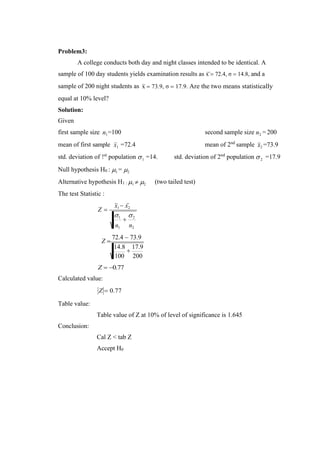
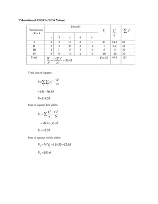
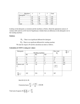
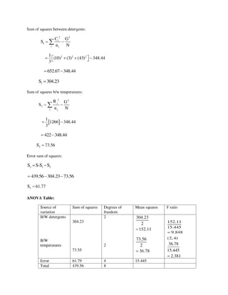
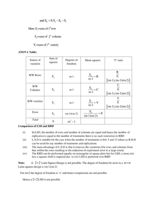
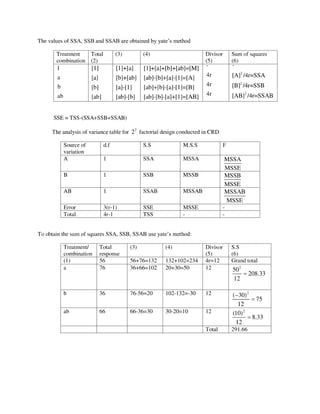
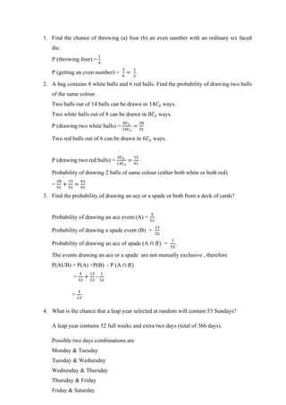
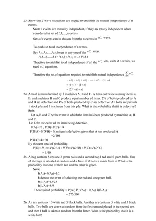
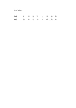
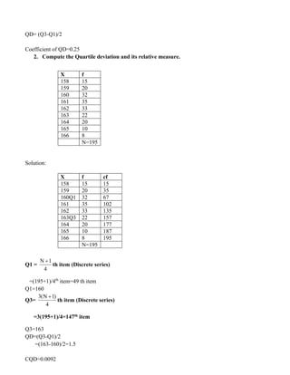
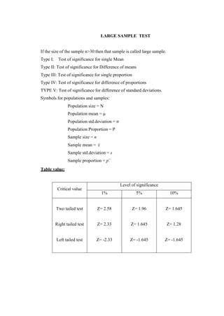
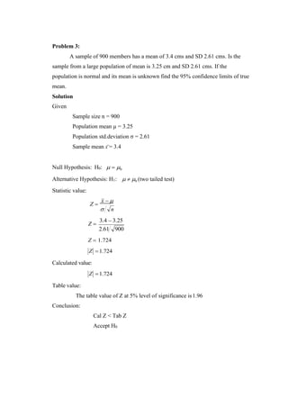
![Example On tossing a coin , either head or tail can occur but not both. i.e occurrence
of head excludes the occurrence of tail. The events of occurrence of head and tail are
mutually exclusive.
Equally likely events
Two events are said to be equally likely events if each one of them has an equal
chance of occurrence.
In tossing an unbiased coin the occurrence of head or tail are equally likely.
Addition law of probability:
If A and B are any two events, and are not disjoint, then
( ) ( ) ( ) ( )
P A B P A P B P A B
= + −
Proof:
From the Venn diagram, the events A and A B
are disjoint.
Therefore ( )
A B A A B
=
( ) [ ( )]
P A B P A A B
=
( ) ( )
P A P A B
= +
Adding and subtracting ( )
P A B
,
( ) ( ) ( ) ( ) ( )
P A B P A P A B P A B P A B
= + + −
( ) [( ) ( )] ( )
P A P A B A B P A B
= + −
( ) ( ) ( ) ( )
P A B P A P B P A B
= + −
Conditional Probability
Ans:The conditional probability of an event B, assuming that the event A has
happened.
( )
( / ) , ( ) 0
( )
P A B
P B A providedP A
P A
=
Similarly, ( )
( / ) , ( ) 0
( )
P A B
P A B providedP B
P B
=
Multiplication law of probability](https://image.slidesharecdn.com/coursematerial-imca-220303195904/85/Course-material-mca-2-320.jpg)
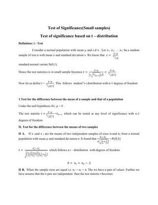
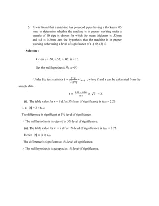
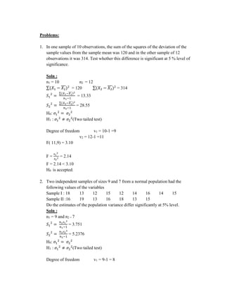
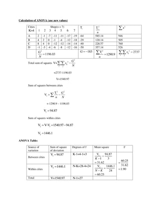
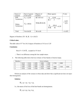
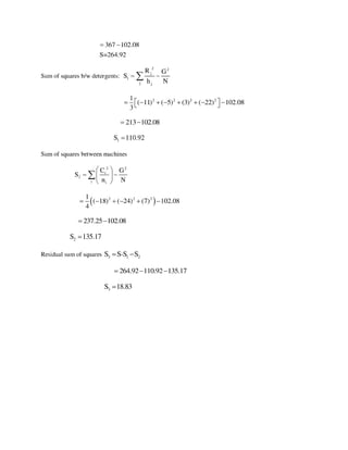
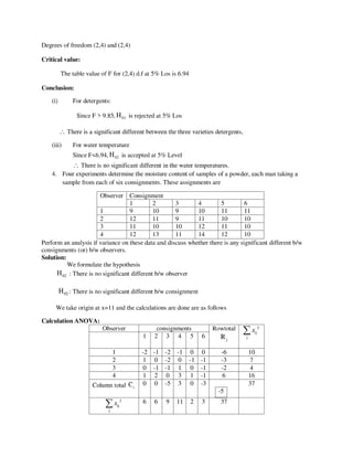
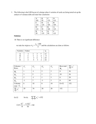
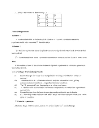
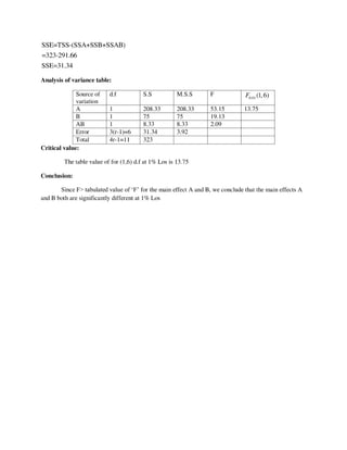
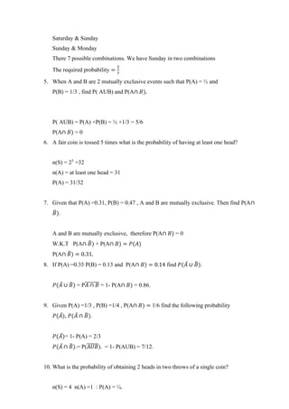
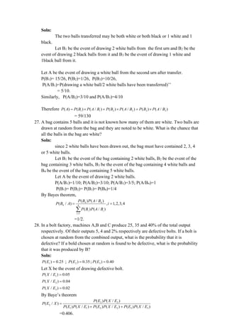
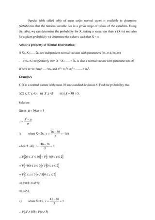
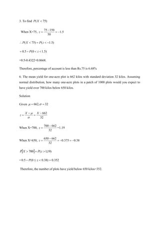
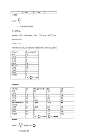
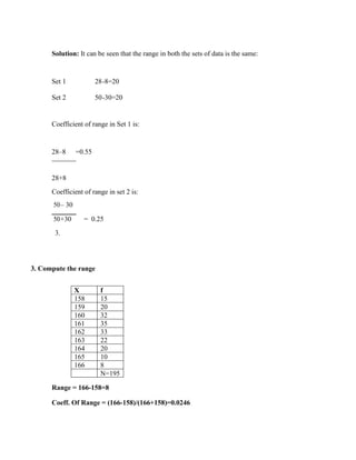
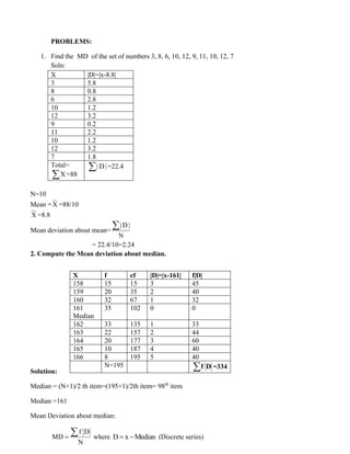
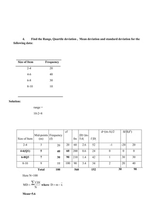
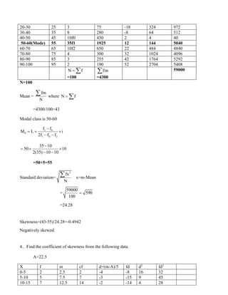
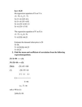
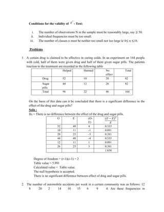
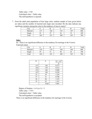
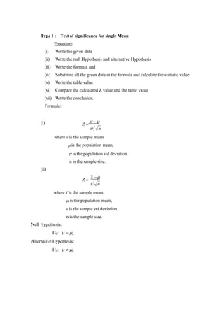
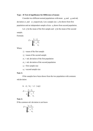
![A real – valued function defined on the outcome of a probability experiment is called
a random variable.
Example :Suppose that a coin is tossed twice so that the sample space is S = {HH, HT,
TH, TT}. Let X represent the number of heads that can come up. With each sample
point we can associate a number for X as shown in Table . Thus, for example, in the
case of HH (i.e., 2 heads), X = 2 while for TH (1 head), X = 1. It follows that X is a
random variable.
Table
Sample
Point
HH HT TH TT
X 2 1 1 0
It should be noted that many other random variables could also be defined on this
sample space, for example, the square of the number of heads or the number of
heads minus the number of tails.
Discrete Random Variable :
A random variable whose set of possible values is either finite or countably infinite is
called discrete random variable.
Example: Number of transmitted bits received in error.
Cumulative Distribution Function :
The cumulative distribution F(x) of a discrete random variable X with probability
distribution f(x) is given by
F(x) = P(X x) =
x
t
f(t) for - < x <
Mean or Expectation of a discrete Random variable X:
Let X be a discrete random variable assuming values x1, x2,…, xn with corresponding
probabilities P1, P2,…, Pn. Then
E(X) =
i
i
i )
p(x
x is called the expected value of X.
E(X) is also commonly called the mean or the expectation of X. A useful identity
states
that for a function g,
E[g(x)] =
i
x
i
i )
p(x
)
g(x
Continuous Random Variable:
A random variable X is said to be continuous if it takes all possible values between
certain limits say from real number ‘a’ to real number ‘b’.
Example: The length of time during which a vacuum tube installed in a circuit
functions is a continuous random variable, number of scratches on a surface,
proposition of defective parts among 1000 tested, number of transmitted in error.](https://image.slidesharecdn.com/coursematerial-imca-220303195904/85/Course-material-mca-4-320.jpg)
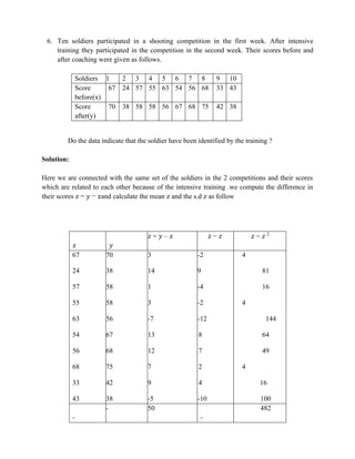
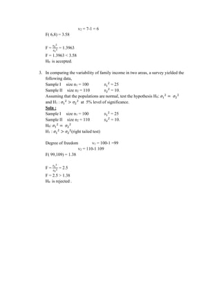
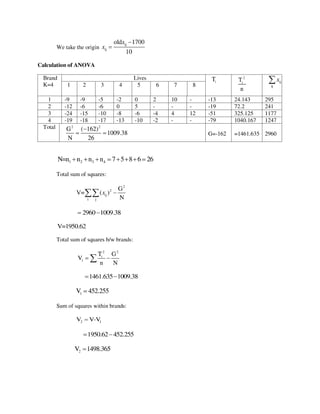
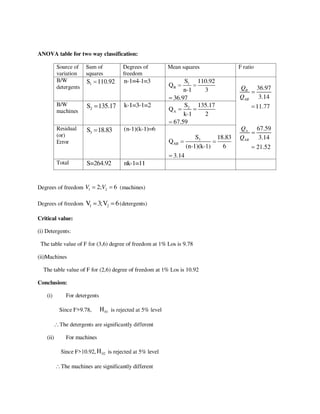
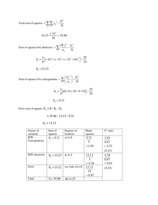
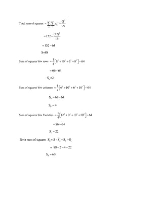
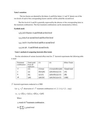
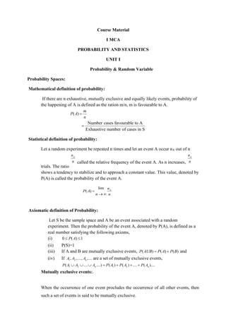
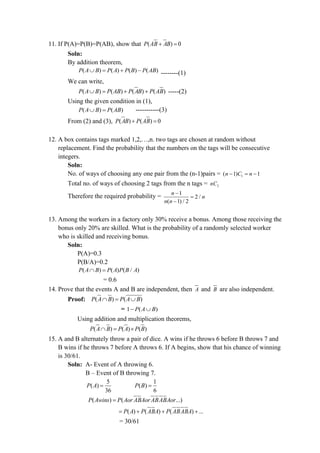
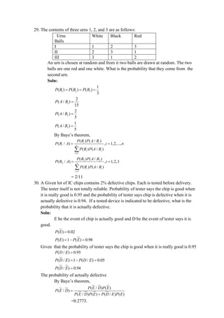
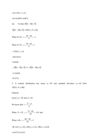
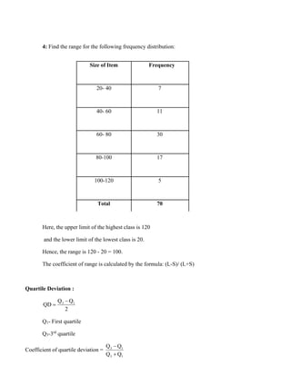
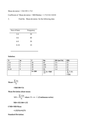
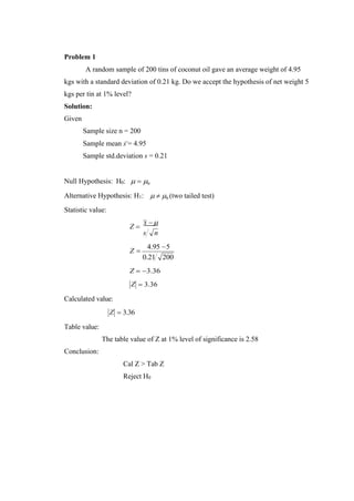
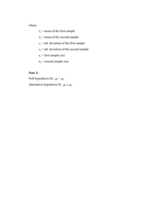
![Cumulative distribution function of a continuous random variable:
The cumulative distribution function of a continuous random variable X is
F(x) = P(X x) = dt
f(t)
x
−
for - < x <
Mean or Expectation of a Continuous Random variable X:
Suppose X is a continuous random variable with probability density function f(x). The
mean or expected value of X, denoted as or E(X) is
= E(X) =
−
dx
f(x)
x
A useful identity is that for any function g,
E[g(x)] =
−
dx
f(x)
g(x)
Variance of X:
The variance of X, denoted as V(X) or 2
, is
2
= V(X) =
−
− dx
f(x)
μ)
(x 2
=
−
− 2
2
μ
dx
f(x)
x
= E[X2
] – [E(X)]2
Moment generating function of a random variable X about the origin:
Moment generating function of a random variable X about the origin is defined as
MX(t) = E[etX
] = x
tx
p(x)
e , if X is discrete
−
dx
(x)
f
e X
tx
, if X is continuous.
Tchebyshev's Inequality:
Let X be a random variable with mean E(X) = and variance 2
var(X) = . Then the
Tchebyshev’s inequality states that
( )
2
2
P X t
t
−
For any t>0.
Other equivalent form can be written for this inequality is
( )
2
2
P X t 1
t
− −
( ) 2
1
P X n
n
−
Problems:](https://image.slidesharecdn.com/coursematerial-imca-220303195904/85/Course-material-mca-5-320.jpg)
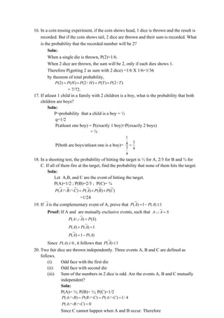
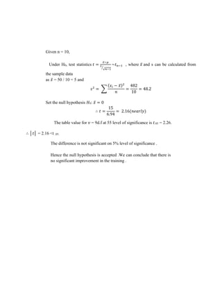
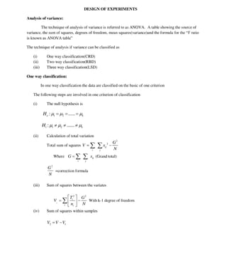
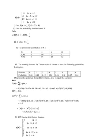
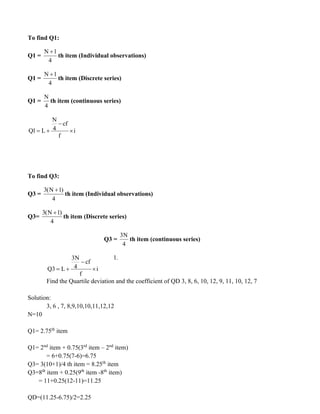
![( ) ( ) ( ) ( )
P A B C P A P B P C
Therefore the events are pairwise independent, but not mutually
independent.
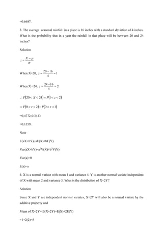
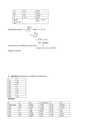
21. Two defective tubes get mixed up with 2 good ones. The tubes are tested, one by one,
until both defectives are found. What is the probability that the last defective tube is
obtained on (i) the second test (ii) the third test and (iii) the fourth test.
Soln:
Let D represent defective and N represent non-defective tube.
(i) P(Second D in the II test)=P(D in the I test and D in the II test)
1 2
( )
P D D
=
1 2
( ) ( )
P D P D
= =1/6
(ii) P(Second D in the III test) 1 2 3 1 2 3
( )
P D N D orN D D
= =1/3
(iii) P(Second D in the IV test)
1 2 3 4 1 2 3 4 1 2 3 4
( ) 1/ 2
P D N N D orN D N D orN N D D
= = =
22. If the events A and B are independent then prove that
(i) A and B are independent.
(ii) A and B are independent.
(iii) A and B are independent.
Proof: (i) by Demorgan’s law
A B A B
=
( ) ( )
P A B P A B
=
1 ( )
P A B
= −
1 [ ( ) ( ) ( )]
P A P B P A B
= − + −
1 [ ( ) ( ) ( )( )]
P A P B P A B
= − + −
( ) ( )
P A P B
=
Therefore A and B are independent.
(ii) the events A B
and A B
are mutually exclusive.
( ) ( )
A B A B B
=
( ) ( ) ( )
P A B P A B P B
+ =
( ) ( ) ( )
P A B P B P A B
= −
( ) ( ) ( ) ( )
P A B P B P A P B
= − +
( ). ( )
P A P B
=
Therefore A and B are independent.
(iii) ( ) ( )
A A B A B
=
( ) ( ) ( )
P A P A B P A B
= +
( ) ( ) ( )
P A B P A P A B
= −
( ) ( )
P A P B
=
Therefore A and B are independent.](https://image.slidesharecdn.com/coursematerial-imca-220303195904/85/Course-material-mca-10-320.jpg)
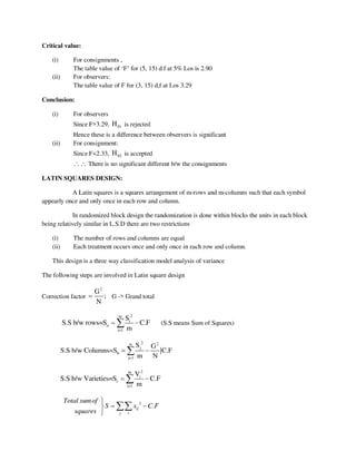
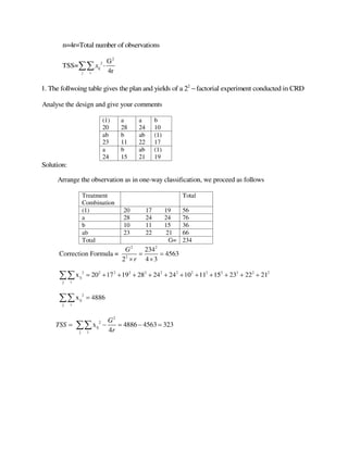
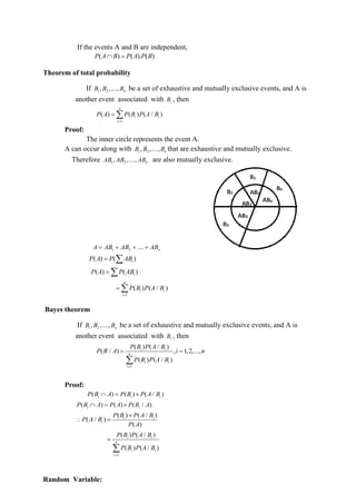
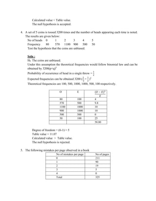
![31. A certain firm has plant A, B and C producing IC chips. Plant A produces twice the
output from B and B produces twice the output from C. The probability of a non-
defective product produced by A,B and C are respectively 0.85, 0.75 and 0.95. A
customer receives a defective product. Find the probability that it came from plant B.
Soln:
P(A)=1; P(B)=0.5; P(C)=0.25
P(E/A)=0.85 ; P(E/B)=0.75 ; P(E/C)=0.95
( / ) 0.15
P E A =
( / ) 0.25
P E B =
( / ) 0.05
P E C =
The probability that the customer receives a defective product from plant B is
( ) ( / )
( / )
( ) ( / ) ( ) ( / ) ( ) ( / )
P B P E B
P B E
P A P E A P B P E B P C P E C
=
+ +
=0.4348
32. There are 3 true coins and 1 false coin with ‘head’ on both sides. A coin is chosen at
random and tossed 4 times. If ‘head’ occurs all the 4 times, what is the probability that
the false coin has been chosen and used?
Soln:
P(T)=P(the coin is a true coin)=3/4
P(F)=P(the coin is a false coin)=1/4
Let A be the event of getting all heads in 4 tosses.
1 1 1 1 1
( / )
2 2 2 2 16
P A T = =
( / ) 1
P A F =
By Baye’ theorem,
( ) ( / )
( / )
( ) ( / ) ( ) ( / )
P F P A F
P F A
P F P A F P T P A T
=
+
= 16/19
33. A coin with is tossed n times. Show that the probability that the number of heads
obtained is even is 0.5 1 ( )n
q p
+ −
.
Soln:
P(even no.of heads are obtained)=P(0 head or 2 head or 4 head or …)
=P(0 head or 2 head or 4 heads or …)
0 2 2 4 4
0 2 4 ...
n n n
nC q p nC q p nC q p
− −
= + + + --------(1)
( ) 0 1 1 2 2 3 3 4 4
0 1 2 3 4 ...
n n n n n n
q p nC q p nC q p nC q p nC q p nC q p
− − − −
+ = + + + + + -------(2)
( ) 0 1 1 2 2 3 3 4 4
0 1 2 3 4 ...
n n n n n n
q p nC q p nC q p nC q p nC q p nC q p
− − − −
− = − + − + + -------(3)
Adding (2) and (3),
1+( )
n
q p
− = 0 2 2 4 4
0 2 4
2[ ...]
n n n
nC q p nC q p nC q p
− −
= + + + --------(4)
Using (4) in (1),
The required probability =0.5 1 ( )n
q p
+ −
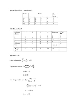
34. Let X be a discrete RV whose cumulative distribution function is](https://image.slidesharecdn.com/coursematerial-imca-220303195904/85/Course-material-mca-14-320.jpg)
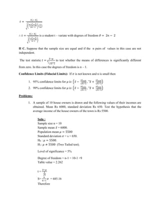
![Find
(i) The probability distribution of X.
(ii) ( )
6
X
2
P
(iii) Mean of X
(iv) Variance of X
Soln:
(i)
(ii) ( )
6
X
2
p
4
X
p =
=
6
1
=
(iii) Mean of X = ( )
= i
i x
p
x
X
E
6
28
=
E(X2
) = 2
i i
i
x p(x )
= 0+12
(1/3)+42
(1/6)+ 62
(2/6)+ 102
(1/6)
= 154/6
(iv)Variance of X = ( )
2
2
X
E
X
E
X
Var −
=
190 784
6 36
= −
356
36
=
9
89
=
37.
If ( )
=
=
=
otherwise
,
0
p.m.f
a
represents
1,2,3,4,5
x
Kx,
x
X
P
(i) Find ‘K’
(ii) Find ( )
number
prime
a
being
X
P
(iii) Find
1
X
/
2
5
X
2
1
P
(iv) Find the distribution function.
Soln:
(i) K+2K+3K+4K+5K=1
15K=1
15
1
K =
(ii) ( )
number
prime
a
being
x
X
P = ( ) ( ) ( )
5
X
P
3
X
P
2
X
P =
+
=
+
=
=
2 3 5 10
15 15 15 15
2
3
= + + =
=
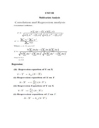
X 0 1 4 6 10
F[x] 0 1/3 ½ 5/6 1
P(X) 0 1/3 1/6 2/6 1/6](https://image.slidesharecdn.com/coursematerial-imca-220303195904/85/Course-material-mca-16-320.jpg)
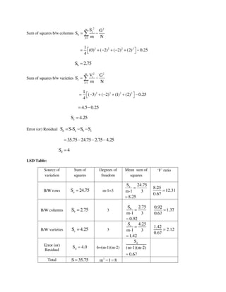
![b) Find the value of (a) C and (b) mean of the following distribution given
( )
( )
−
=
otherwise
0
1
x
0
for
x
x
C
x
f
2
Soln:
a) ( )
=
4
2
dx
x
f
4
X
p
27
2
k =
27
16
4]
P[X =
b) C = 6
Mean = E[X] =
2
1
40. A continuous r.v. has the pdf of f(x) = kx4
; –1 < x < 0. Find the value of k and also
−
−
4
1
/X
2
1
X
P
Soln:
k = 5
−
−
4
1
/X
2
1
X
P = 0.0303
41. A random variable X has density function given by
=
otherwise
0
k
x
0
for
k
1
f(x)
Find (i) m.g.f. (ii) rth
moment (iii) mean (iv) variance.
Soln:
MX(t) = 1 + ...
1)!
(r
(kt)
...
2!
kt r
+
+
+
Coefficient of tr
=
1)!
(r
Kr
+
Mean =
2
K
Variance =
12
K2
42. The first four moments of a distribution about X = 4 is 1, 4, 10 and 45 respectively.
Show
that the mean is 5, variance is 3, 3 = 0 and 4 = 26.
Soln:](https://image.slidesharecdn.com/coursematerial-imca-220303195904/85/Course-material-mca-18-320.jpg)
![Mean = A + '
μ1
= 5
(Variance) 2 = '
μ2
– 2
1 '
μ = 3
3 = '
μ3 – 3 '
μ2 '
μ1
+ 2 3
1 '
μ = 0
4 = '
μ4
+ 4 '
μ3 '
μ1
+ 6 '
μ2
2
1 '
μ – 3 4
1 '
μ = 26
43. Find the probability distribution of the total number of heads obtained in four tosses
of a
balanced coin. Hence the MGP of X, mean of X and variance of X.
Soln:
MX(t) = E[etX
] = x
tx
p(x)
e , if X is discrete
MX(t) =
16
1
[1 + 4et
+ 6e2t
+ 4e3t
+ e4t
]
E[X] = 2
Variance[X] = E(X2
) – [E(X)]2
= 1
PROBABILITY DISTRIBUTIONS
Introduction
While constructing probabilistic models for observable phenomena, certain
probability distributions arise more frequently than do others. we treat such distributions that
play important roles in many engineering applications as special probability distributions.
DISCRETE DISTRIBUTIONS
Bernoulli Trials and Bernoulli Distributions
Let A be an event ((trail) associated with a random experiment such that p(A) remains
the same for the repetitions of that random experiment, then the events are called Bernoulli
trails.
A random variable X which takes only two values either 1 (success) or 0(failure) with
probability p and q respectively. i.e., P(X=1)=p, P(X=0)=q, p+q=1 is called Bernoulli variate
and is said to have a Bernoulli distribution.
X: Number of heads in 4 tosses of a coin
x: 0 1 2 3 4
p(x):
16
1
16
4
16
6
16
4
16
1](https://image.slidesharecdn.com/coursematerial-imca-220303195904/85/Course-material-mca-19-320.jpg)
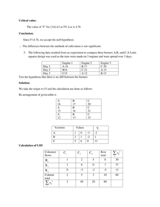
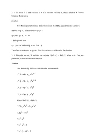
![1. The mean and variance of a binomial distribution are 4 and 4/3 respectively. Find P(X≥1)
if n=6.
Solution
Mean of binomial distribution = np = 4
Variance of binomial distribution = npq = 4/3
4
3
4
=
np
npq
3
1
=
q
Now p = 1-q = 1-1/3 = 2/3
Given n=6
x
n
x
c q
p
n
x
X
P x
−
=
= )
(
]
1
[
1
)
1
(
−
=
X
P
X
P
]
0
[
1 =
−
= X
P
0
6
0
0
6
1 −
−
= q
p
c
6
1 q
−
=
6
)
3
1
(
1−
=
729
1
1−
=
729
728
=
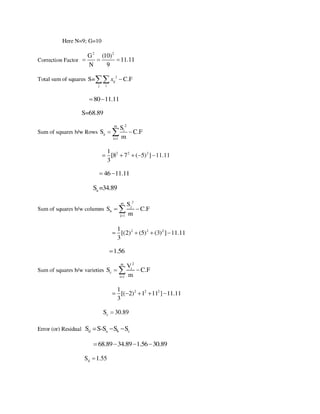
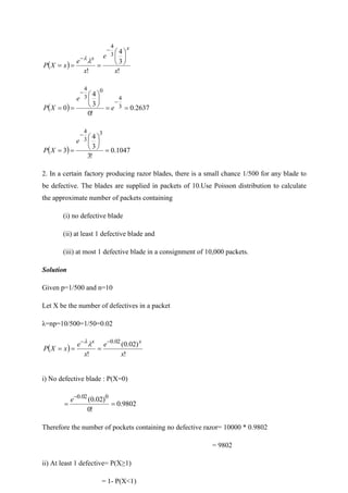
2. The mean and variance of binomial distributions are 4 and 3 respectively. Find P(X=0),
P(X=1) and P(X≥2).
Solution](https://image.slidesharecdn.com/coursematerial-imca-220303195904/85/Course-material-mca-23-320.jpg)
![Mean of binomial distribution = np = 4
Variance of binomial distribution = npq= 3
4
3
=
np
npq
4
3
=
q
Now p = 1-q = 1-3/4 = 1/4
Since Mean = np = 4
= n(1/4) = 4
n = 16
x
n
x
c q
p
n
x
X
P x
−
=
= )
(
n
c q
p
n
X
P 0
0
)
0
( =
=
16
)
4
3
(
16 0
c
=
01
.
0
)
4
3
( 16
=
=
1
1
1
)
1
( −
=
= n
c q
p
n
X
P
15
1
1
16 q
p
c
=
053
.
0
)
4
3
)(
4
1
(
16 15
=
=
)
2
(
1
)
2
(
−
=
X
P
X
P
)]
1
(
)
0
(
[
1 =
+
=
−
= X
P
X
P
063
.
0
1
]
053
.
0
01
.
0
[
1 −
=
+
−
=
937
.
0
=](https://image.slidesharecdn.com/coursematerial-imca-220303195904/85/Course-material-mca-24-320.jpg)
![0
)
2
1
(
9 2
2
=
−
+
− p
p
p
0
2
1
9 2
2
=
+
−
− p
p
p
0
1
2
8 2
=
−
+ p
p
16
32
4
2 +
−
=
p
16
6
2
−
=
p 16
8
,
16
4 −
=
2
1
,
4
1 −
=
p
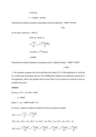
Since p cannot be negative, p=1/4.
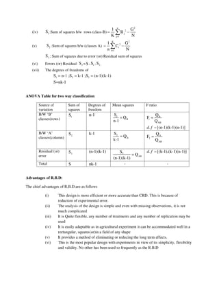
4. Out of 800 families with 4 children each, how many families would be expected to have
(i) 2 boys and 2 girls
(ii) at least 1 boy
(iii) at most 2 girls and
(iv) children of both sexes.
Assume equal probabilities for boys and girls.
Solution
Considering each child is a trial, n=4. Assuming that birth of a boy is success, p = 1/2
and q = ½
Let X denote the number of successes (boys)
(i) P[2 boys and 2 girls] = P(X=2)
x
n
x
c q
p
n
x
X
P x
−
=
= )
(
2
4
2
)
2
1
(
)
2
1
(
4
)
2
( 2
−
=
= c
X
P](https://image.slidesharecdn.com/coursematerial-imca-220303195904/85/Course-material-mca-26-320.jpg)
![8
3
)
2
1
(
6 4
=
=
Therefore number of families having 2 boys and 2 girls=N[P(X=2)]
= 800(3/8) = 100 * 3
= 300
(ii) P[ at least 1 boy ] = P[X≥1]
= P[X=1] + P[X=2] + P[X=3] + P[X=4]
=1- P[X=0]
0
4
0
)
2
1
(
)
2
1
(
4
)
0
( 0
−
=
= c
X
P
16
15
)
2
1
(
1
)
0
(
1 4
=
−
=
=
− X
P
Therefore number of families having at least 1 boy = N [1-(P(X=0)]
= 800 (15/16) = 750
(iii) P( at most 2 girls )= P(exactly 0 girl, 1 girl or 2 girls)
= P[ X=4, X=3, X=2]
= 1-[ P(X=0) + P(X=1) ]
+
−
= −
− 1
4
1
0
4
0
)
2
1
(
)
2
1
(
4
)
2
1
(
)
2
1
(
4
1 1
0 c
c
16
5
1
)
16
4
16
1
(
1
)
2
1
(
4
)
2
1
(
1 4
4
−
=
+
−
=
+
−
=
16
11
=
Therefore number of families having at most 2 girls = N[P(X≥2)]
= 800 (11/16) = 550
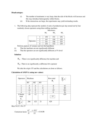
(iv) P[ children of both sexes] = 1 – P[ children of same sex]
= 1 –[ P( all are boys) + P( all are girls)]](https://image.slidesharecdn.com/coursematerial-imca-220303195904/85/Course-material-mca-27-320.jpg)
![= 1- [P(X=4) + P(X=0)]
]
)
2
1
(
)
2
1
[(
1
)
2
1
(
)
2
1
(
4
)
2
1
(
4
1 4
4
4
0
4
0
4
+
−
=
+
−
= c
c
= 1- 2/16 = 7/8
Therefore number of families having children of both sexes = 800 * 7/8
= 700
5. An irregular 6 faced die is such that the probability that it gives 3 even numbers in 5 throws
is twice the probability that it gives 2 even numbers in 5 throws. How many sets of exactly 5
trials can be expected to give no even number out of 2500 sets.
Solution
Let the probability of getting an even number with the unfair die bep .
Let X denote the number of even numbers obtained in 5 trials (throws)
Given: P(X=3) = 2 * P(X=2)
3
2
2
3
2
3
5
*
2
5 q
p
q
p c
c =
p = 2q
p = 2(1-p)
3p = 2
P = 2/3
q=1-p = 1/3
Now P[ getting no even number ] = P[X=0]
243
1
)
3
1
(
5 5
5
0
0
=
=
q
p
c
Therefore number of sets having no success ( even number) out of N sets = N [ P(X=0) ]
= 2500 * 1/243
= 10 nearly](https://image.slidesharecdn.com/coursematerial-imca-220303195904/85/Course-material-mca-28-320.jpg)
![7.. Assuming that half of the population is vegetarian and that 100 investigators each take 10
individuals to see whether they are vegetarians, how many would you expect to report that 3
people or less were vegetarians?
Solution
n=10, p=1/2, q=1/2
x
n
x
c q
p
n
x
X
P x
−
=
= )
(
x
x
cx
−
= 10
)
2
1
(
)
2
1
(
10
10
)
2
1
(
10 x
c
=
)
3
(
)
2
(
)
1
(
)
0
(
)
3
( =
+
=
+
=
+
=
=
X
P
X
P
X
P
X
P
X
P
10
10
10
10
)
2
1
(
10
)
2
1
(
10
)
2
1
(
10
)
2
1
(
10 3
2
1
0 c
c
c
c +
+
+
=
]
120
45
10
1
[
)
2
1
( 10
+
+
+
=
1718
.
0
1024
176
]
176
[
)
2
1
( 10
=
=
=
Among 100 investigators, the number of investigators who report that 3 or less were
consumers
=100 * 0.1718
=17 investigators
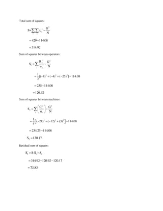
14. A factory produces 10 articles daily. It may be assumed that there is a constant probability
p= 0.1 of producing a defective article. Before the articles are stored, they are inspected and
the defective ones are set aside. Suppose that there is a constant probability r = 0.1, that a
defective article is misclassified. If X denote the number of articles classified as defective at
the end of a production day, find a) P(X=3) and b) P(X>3)
Solution
Let X be the random variable represented by the number of articles which are
defective.](https://image.slidesharecdn.com/coursematerial-imca-220303195904/85/Course-material-mca-29-320.jpg)
![P[ a defective article is classified as defective ] = P( an article produced is defective) *P( it is
classified as defective)
= 0.1 *0.9
p = 0.09
q = 1 – p = 0.91
n= 10
x
n
x
c q
p
n
x
X
P x
−
=
= )
(
x
x
cx
−
= 10
)
91
.
0
(
)
09
.
0
(
10
7
3
)
91
.
0
(
)
09
.
0
(
10
)
3
( 3
c
X
P =
=
0452
.
0
=
)
3
(
1
)
3
(
−
=
X
P
X
P
)]
3
(
)
2
(
)
1
(
)
0
(
[
1 =
+
=
+
=
+
=
−
= X
P
X
P
X
P
X
P
]
)
91
.
0
(
)
09
.
0
(
10
)
91
.
0
(
)
09
.
0
(
10
)
91
.
0
(
)
09
.
0
(
10
)
91
.
0
(
)
09
.
0
(
10
[
1 7
3
8
2
9
1
10
0
3
2
1
0 c
c
c
c +
+
+
−
=
=0.0089
POISSON DISTRIBUTION
Definition
If X is a discrete random variable that assumes only non-negative values such that its
probability mass function is given by
( )
otherwise
,
0
0
where
.
0,1,2,3,..
x
,
!
=
=
=
=
−
x
e
x
X
P
x
then X is said to follow Poisson distribution with the parameter .
Poisson Distribution is a Limiting case of Binomial Distribution](https://image.slidesharecdn.com/coursematerial-imca-220303195904/85/Course-material-mca-30-320.jpg)
![Suppose in a binomial distribution,
1. The number of trails n is indefinitely large, i.e.,
→
n .
2. The probability of success p for each trail is very small, i.e, 0
→
p .
3. )
(
=
np is finite and
n
p
= ,
n
p
q
−
=
−
= 1
1 where is a positive constant.
Mean of the Poisson distribution
Mean =
=
=
=
0
)
(
)
(
x
x
X
xP
X
E
=
−
=
0
!
x
x
x
e
x
!
1
1
x
x
e
x
x
−
=
−
=
=
−
−
−
=
1
1
)!
1
(
x
x
x
e
=
= −
e
e
Mean
Variance of Poisson distribution
2
2
)]
(
[
)
(
Var(X) X
E
X
E −
=
=
=
0
2
2
)
(
)]
(
[
x
x
p
x
X
E
=
−
=
0
2
!
x
x
x
e
x
=
−
−
+
=
0
2
!
)
(
x
x
x
e
x
x
x
=
−
+
−
=
0
!
)
)
1
(
(
x
x
x
e
x
x
x
](https://image.slidesharecdn.com/coursematerial-imca-220303195904/85/Course-material-mca-31-320.jpg)
![!
!
)
1
(
0
0
x
e
x
x
e
x
x
x
x
x
x
−
=
=
−
+
−
=
=
−
=
−
−
+
−
=
1
2
)!
1
(
)!
2
( x
x
x
x
x
e
x
e
=
−
−
=
−
−
−
+
−
=
1
1
2
2
2
)!
1
(
)!
2
( x
x
x
x
x
e
x
e
=
−
−
=
−
−
−
+
−
=
1
1
2
2
2
)!
1
(
)!
2
( x
x
x
x
x
e
x
e
e
e
e
e −
−
+
= 2
+
= 2
2
)
(X
E
=
−
+
=
−
= 2
2
2
2
)]
(
[
)
(
Var(X) X
E
X
E
Therefore variance of the poisson distribution is λ
Examples:
1.If X is a Poisson variate such that P(X=1)=3/10 and P(X=2)=1/5. Find P(X=0) and P(X=3)
Solution
( )
!
x
e
x
X
P
x
−
=
=
( ) (1)
10
3
!
1
1
1
=
=
=
−
e
X
P
( ) (2)
5
1
!
2
2
2
=
=
=
−
e
X
P
10
3
5
1
!
1
!
2
e
)
1
(
)
2
(
2
-
=
−
e
3
4
3
2
2
)
1
(
)
2
(
=
=
](https://image.slidesharecdn.com/coursematerial-imca-220303195904/85/Course-material-mca-32-320.jpg)
![0025
.
0
!
0
6
)
0
(
0
6
=
=
=
−
e
X
P
)]
2
(
)
1
(
)
0
(
[
1
)
3
(
1
)
3
( =
+
=
+
=
−
=
−
=
X
P
X
P
X
P
X
P
X
P
9380
.
0
)
18
6
1
(
1 6
=
+
+
−
= −
e
8. A car hire firm has 2 cars which it hires out day by day. The number of demands for a car
on each day follows a Poisson distribution with mean 1.5. Calculate the proportion of days on
which
i) neither car is used
ii) some demand is not fulfilled
Solution
Let X be random variable representing the number of demands for cars:
P( x demands in a day)=
!
)
(
x
e
x
X
P
x
−
=
=
Given: λ = 1.5
Now
!
)
5
.
1
(
)
(
5
.
1
x
e
x
X
P
x
−
=
=
i) the proportion of days on which neither car is used
2231
.
0
!
0
5
.
1
)
0
( 5
.
1
0
5
.
1
=
=
=
= −
−
e
e
X
P
ii) The proportion of days on which some demand is refused
The demand is refused when x is more than 2
)]
2
(
[
1
)
2
(
−
=
X
P
X
P
)]
2
(
)
1
(
)
0
(
[
1 =
+
=
+
=
−
= X
P
X
P
X
P
]
!
2
)
5
.
1
(
!
1
)
5
.
1
(
!
0
)
5
.
1
(
[
1
2
5
.
1
1
5
.
1
0
5
.
1 −
−
−
+
+
−
=
e
e
e
19126
.
0
=](https://image.slidesharecdn.com/coursematerial-imca-220303195904/85/Course-material-mca-36-320.jpg)
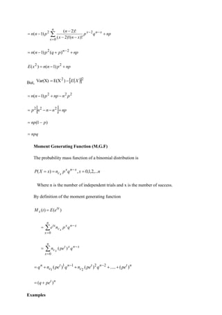
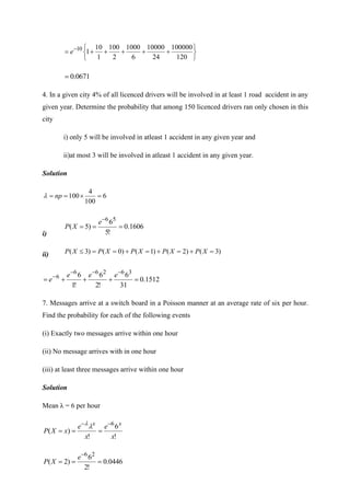
![9. The proofs of a 500 page book contains 500 misprints. Find the probability that there are at
least 4 misprints in a randomly chosen page.
Solution
Total number of mistakes= 500
Total number of pages= 500
The average number of mistake per page is 1. λ =1
Let X be a random variable of number of mistakes in a page.
!
1
!
)
(
1
x
e
x
e
x
X
P
x
x −
−
=
=
=
)
4
(
mistakes)
4
least
at
P(
= X
P
)
4
(
1
−
= X
P
)]
3
(
)
2
(
)
1
(
)
0
(
[
1 =
+
=
+
=
+
=
−
= X
P
X
P
X
P
X
P
+
+
+
−
=
−
−
−
−
!
3
!
2
!
1
!
0
1
1
1
1
1
e
e
e
e
+
+
+
−
= −
6
1
2
1
1
1
1 1
e
0180
.
0
=
NORMAL DISTRIBUTION
Definition
A normal distribution is a continuous distribution given by
2
2
1
2
1
−
−
=
x
e
y where X is
a continuous normal variate distributed with density function
2
2
1
2
1
)
(
−
−
=
x
e
f with mean and standard deviation .
Deviation of the distribution](https://image.slidesharecdn.com/coursematerial-imca-220303195904/85/Course-material-mca-37-320.jpg)
![(OR)
Mode = Mean - 3 Mean + 3 Median
(OR)
Mode = 3 Median - 2 Mean
Problems :
1.Find the AM , median and mode of the following set of observations:
25,32,28,34,24,31,36; 27,29,30.
Mean=
x
n
=(25+32+28+34+24+31+36+ 27+29+30)/10=296/10
=29.6
24,25,27,28,29,30,31,32,34,36
Median =(n+1)/2th item
=(10+1)/2 th item=5.5th
item
5.5th
item =(5th
item+6th
item)/2=(29+30)/2=29.5
There is no mode.
2. Find the mode of following data: 2,3,2,1,3,2,3,3,2,1,3,3,3,2,2,1,1,3,3,3
Mode =3 [ since 3 come more number of times ]
3. Find the mean, median and mode.
x f
155 30
156 20
157 5
158 5
159 10
160 15
161 5
162 10
Solution:
x f fx cf(cumulative
frequency)
155(mode) 30 4650 30
156 20 3120 50
157(Median) 5 785 55
158 5 790 60
159 10 1590 70
160 15 2400 85
161 5 805 90
162 10 1620 100
N f
= fx
](https://image.slidesharecdn.com/coursematerial-imca-220303195904/85/Course-material-mca-47-320.jpg)


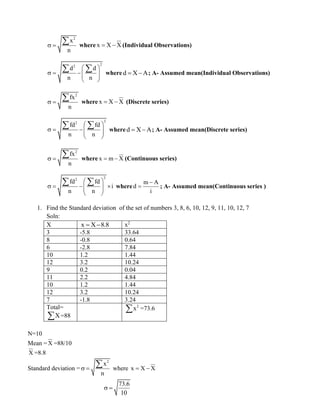

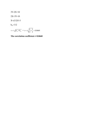
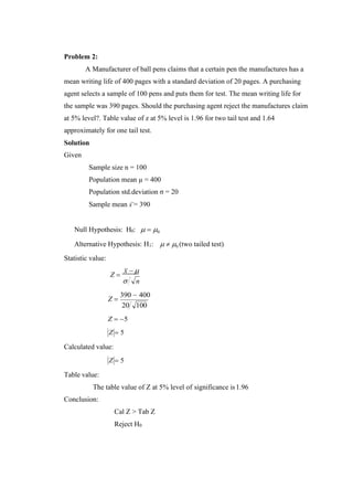
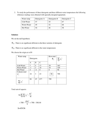
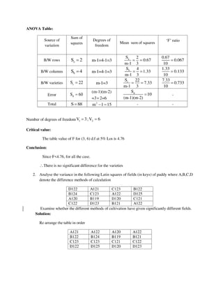
![(400)2
+
(550)2
400 400
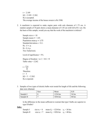
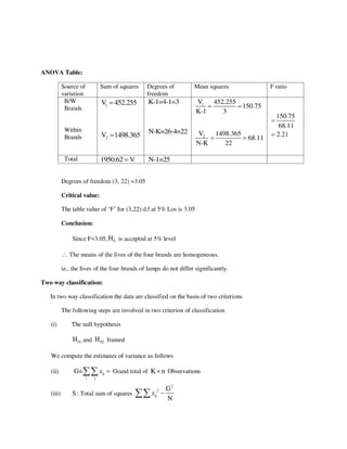
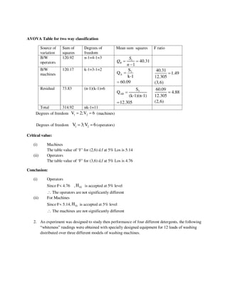
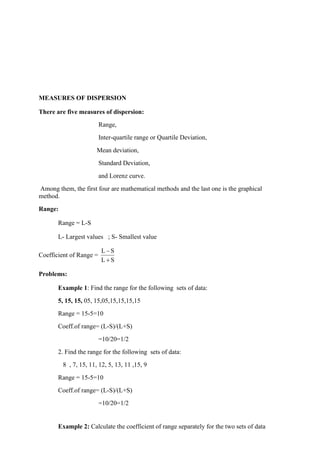
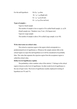
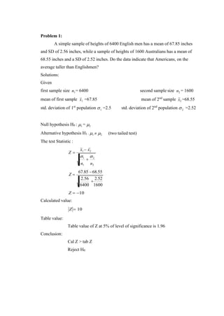
Problem 2:
The sales manager of a large company conducted a sample survey in states A
and B taking 400 samples in each case. The results were in the following table.
State A State B
Average sales Rs. 2,500 Rs. 2,200
S.D. Rs. 400 Rs. 550
Test whether the average sales in the same in the 2 states at 1 % level.
Solution:
n1 = 400 , x1 =2500 , s1 = 400
n2 = 400 , x2 =2200 , s2 = 550
H 0 : 1
= 2
H1 : 1
2 [ two tailed test ]
The test statistic
Z =
(x1−x2 )
=
2500− 2000
= 8.82
Calculated value:
Z = 8.82
Table value:
Conclusion:
Table value of Z at 1% of level of significance is 2.58
Cal Z > tab Z
Reject H0
s 2 s 2
n1 n2
1 + 2](https://image.slidesharecdn.com/coursematerial-imca-220303195904/85/Course-material-mca-94-320.jpg)