Downloaded 21 times

![Sampling Process 1
Let ga (t) be a continuous-time (CT) signal that is sampled
uniformly at t = nT , generating the sequence g[n],
g[n] = ga (nT ), −∞ < n < ∞ (1)
where T is the sampling period and n is an integer.
TELE3113 - Pulse Modulation. Sept. 1, 2009. – p.3/1](https://image.slidesharecdn.com/tele3113wk7tue-110604233606-phpapp01/85/Tele3113-wk7tue-4-320.jpg)
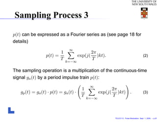
![Sampling Process 2
Sampling
ga(t) g[n]
ga(t) gp(t)
p(t)
∞
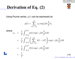
p(t) is a periodic impulse train: p(t) = n=−∞ δ(t − nT ).
TELE3113 - Pulse Modulation. Sept. 1, 2009. – p.4/1](https://image.slidesharecdn.com/tele3113wk7tue-110604233606-phpapp01/85/Tele3113-wk7tue-5-320.jpg)
![FT of Sampled Signal
Assume Ga (jω) ⇔ ga (t), i.e., Ga (jω) = F [ga (t)]. From the
frequency-shifting property of the FT, we have
2π 2π
F [ga (t) · exp(j( )kt)] = Ga (j(ω − k )). (4)
T T
Next, taking FT on both sides of (3) and using (4), we get
∞
1
Gp (jω) = F [gp (t)] = Ga (j(ω − kωT )), −∞ < k < ∞ (5)
T
k=−∞
2π
where ωT = T denotes the angular sampling frequency.
TELE3113 - Pulse Modulation. Sept. 1, 2009. – p.6/1](https://image.slidesharecdn.com/tele3113wk7tue-110604233606-phpapp01/85/Tele3113-wk7tue-7-320.jpg)

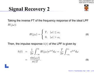
![Signal Recovery 1
Question: Suppose that g[n] is obtained by uniformly sampling
a bandlimited analog signal ga (t) with a highest frequency ωm at
a sampling rate ωT = 2π satisfying (6), can the original analog
T
signal ga (t) be fully recovered from the given sequence g[n]?
Answer: YES, ga (t) can be fully recovered by generating an
impulse train gp (t) and then passing gp (t) through an ideal low
pass filter (LPF) H(jω) with a gain T and a cutoff frequency ω c
satisfying ωm < ωc < ωT − ωm .
∧
g[n] gp(t) LPF g a(t)
TELE3113 - Pulse Modulation. Sept. 1, 2009. – p.8/1](https://image.slidesharecdn.com/tele3113wk7tue-110604233606-phpapp01/85/Tele3113-wk7tue-9-320.jpg)

![Signal Recovery 3
Consider the impulse train gp (t) be expressed as
∞
gp (t) = ga (t) · p(t) = ga (t) · δ(t − nT )
n=−∞
∞ ∞
= ga (nT )δ(t − nT ) = g[n]δ(t − nT ). (10)
n=−∞ n=−∞
Therefore, the output of the LPF is given by the convolution of
gp (t) with the impulse response h(t):
∞
ga (t) =
ˆ g[n]h(t − nT ). (11)
n=−∞
TELE3113 - Pulse Modulation. Sept. 1, 2009. – p.11/1](https://image.slidesharecdn.com/tele3113wk7tue-110604233606-phpapp01/85/Tele3113-wk7tue-12-320.jpg)
![Signal Recovery 4
Substituting h(t) from (9) in (11) and assuming for simplicity
ωc = ωT /2 = π/T , we arrive at
∞
sin[π(t − nT )/T ]
ga (t) =
ˆ g[n]
n=−∞
π(t − nT )/T
∞
t − nT
= g[n] · sinc( ), (12)
n=−∞
T
where sinc(x) is defined as sinc(x) = sin(πx)/(πx).
The reconstructed analog signal ga (t) is obtained by shifting in
ˆ
time the impulse response of the LPF h(t) by an amount nT and
scaling it an amplitude by the factor g[n] for −∞ < n < ∞ and
then summing up all shifted versions.
TELE3113 - Pulse Modulation. Sept. 1, 2009. – p.12/1](https://image.slidesharecdn.com/tele3113wk7tue-110604233606-phpapp01/85/Tele3113-wk7tue-13-320.jpg)

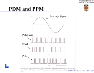

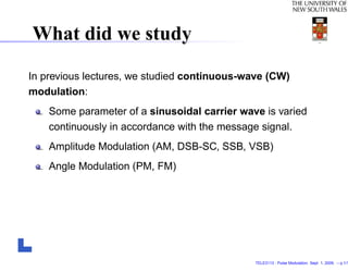
This document discusses pulse modulation techniques in communications. It begins by reviewing continuous-wave modulation techniques studied previously, such as amplitude modulation and angle modulation. It then previews that pulse modulation will be studied next, including analog pulse modulation where a pulse feature varies continuously with the message, and digital pulse modulation using a sequence of coded pulses. The document provides explanations and equations regarding sampling of continuous-time signals, the sampling theorem, and recovery of the original analog signal from its samples. It also introduces pulse amplitude modulation (PAM) using natural and flat-top sampling, as well as pulse duration modulation (PDM) and pulse position modulation (PPM).