These slides provide the basics of Linear Programming

1. Linear Programming
Neil Laws
TT 2010
1.1
1 Introduction
A general optimization problem is of the form: choose x to
maximise f(x)
subject to x ∈ S
where
x = (x1, . . . , xn)T ,
f : Rn → R is the objective function,
S ⊂ Rn is the feasible set.
We might write this problem:
max
x
f(x) subject to x ∈ S.
1.2
For example
• f(x) = cT x for some vector c ∈ Rn,
• S = {x : Ax b} for some m × n matrix A and some
vector b ∈ Rm.
If f is linear and S ⊂ Rn can be described by linear
equalities/inequalities then we have a linear programming (LP)
problem.
If x ∈ S then x is called a feasible solution.
If the maximum of f(x) over x ∈ S occurs at x = x∗ then
• x∗ is an optimal solution, and
• f(x∗) is the optimal value.
1.3
Questions
In general:
• does a feasible solution x ∈ S exist?
• if so, does an optimal solution exist?
• if so, is it unique?
1.4

2. Example
A company produces drugs A and B using machines M1 and
M2.
• 1 ton of drug A requires 1 hour of processing on M1 and 2
hours on M2
• 1 ton of drug B requires 3 hours of processing on M1 and 1
hour on M2
• 9 hours of processing on M1 and 8 hours on M2 are
available each day
• Each ton of drug produced (of either type) yields £1
million profit
To maximise its profit, how much of each drug should the
company make per day?
1.5
Solution
Let
• x1 = number of tons of A produced
• x2 = number of tons of B produced
P1 : maximise x1 + x2 (profit in £ million)
subject to x1 + 3x2 9 (M1 processing)
2x1 + x2 8 (M2 processing)
x1, x2 0
1.6
x1
x2
x1 + 3x2 = 92x1 + x2 = 8
x1 + x2 = 5
The shaded region is the feasible set for P1. The maximum
occurs at x∗ = (3, 2) with value 5.
1.7
Diet problem
A pig-farmer can choose between four different varieties of food,
providing different quantities of various nutrients.
food required
1 2 3 4 amount/wk
A 1.5 2.0 1.0 4.1 4.0
nutrient B 1.0 3.1 0 2.0 8.0
C 4.2 1.5 5.6 1.1 9.5
cost/kg £5 £7 £7 £9
The (i, j) entry is the amount of nutrient i per kg of food j.
1.8

3. Problem P2:
minimise 5x1 + 7x2 + 7x3 + 9x4
subject to 1.5x1 + 2x2 + x3 + 4.1x4 4
x1 + 3.1x2 + 2x4 8
4.2x1 + 1.5x2 + 5.6x3 + 1.1x4 9.5
x1, x2, x3, x4 0
1.9
General form of the diet problem
Foods j = 1, . . . , n, nutrients i = 1, . . . , m.
Data:
• aij = amount of nutrient i in one unit of food j
• bi = required amount of nutrient i
• cj = cost per unit of food j
Let xj = number of units of food j in the diet.
The diet problem is
minimise c1x1 + · · · + cnxn
subject to ai1x1 + · · · + ainxn bi for i = 1, . . . , m
x1, . . . , xn 0.
1.10
In matrix notation the diet problem is
min
x
cT
x subject to Ax b, x 0.
Note that our vectors are always column vectors.
We write x 0 to mean xi 0 for all i. (0 is a vector of zeros.)
Similarly Ax b means (Ax)i bi for all i.
1.11
Real applications
“Programming” = “planning”
Maybe many thousands of variables or constraints
• Production management: realistic versions of P1, large
manufacturing plants, farms, etc
• Scheduling, e.g. airline crews:
• need all flights covered
• restrictions on working hours and patterns
• minimise costs: wages, accommodation, use of seats by
non-working staff
shift workers (call centres, factories, etc)
• Yield management (airline ticket pricing: multihops,
business/economy mix, discounts, etc)
• Network problems: transportation capacity planning in
telecoms networks
• Game theory: economics, evolution, animal behaviour
1.12

4. Free variables
Some variables may be positive or negative, e.g. omit the
constraint x1 0.
Such a free variable can be replaced by
x1 = u1 − v1
where u1, v1 0.
1.13
Slack variables
In P1 we had
maximise x1 + x2
subject to x1 + 3x2 9
2x1 + x2 8
x1, x2 0.
We can rewrite by
maximise x1 + x2
subject to x1 + 3x2 + x3 = 9
2x1 + x2 + x4 = 8
x1, . . . , x4 0.
• x3 = unused time on machine M1
• x4 = unused time on machine M2
x3 and x4 are called slack variables.
1.14
With the slack variables included, the problem has the form
max
x
cT
x subject to Ax = b
x 0.
1.15
Two standard forms
In fact any LP (with equality constraints, weak inequality
constraints, or a mixture) can be converted to the form
max
x
cT
x subject to Ax = b
x 0
since:
• minimising cT x is equivalent to maximising −cT x,
• inequalities can be converted to equalities by adding slack
variables,
• free variables can be replaced as above.
1.16

5. Similarly, any LP can be put into the form
max
x
cT
x subject to Ax b
x 0
since e.g.
Ax = b ⇐⇒
Ax b
−Ax −b
(more efficient rewriting may be possible!).
So it is OK for us to concentrate on LPs in these forms.
1.17
Remark
We always assume that the underlying space is Rn.
In particular x1, . . . , xn need not be integers. If we restrict to
x ∈ Zn we have an integer linear program (ILP).
ILPs are in some sense harder than LPs. Note that the optimal
value of an LP gives a bound on the optimal value of the
associated ILP.
1.18
1.19 1.20

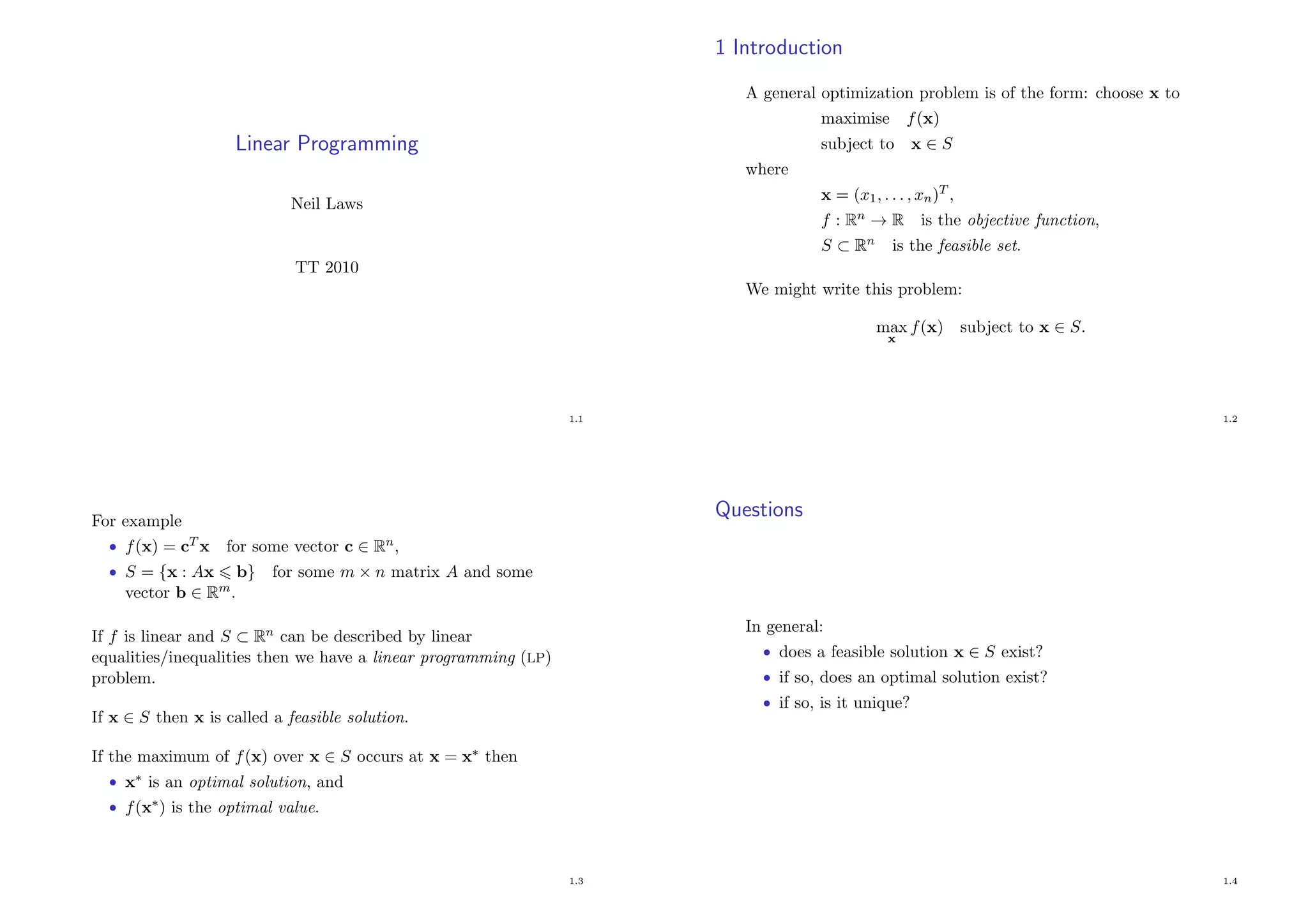
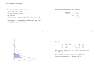
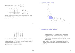
6. 2 Geometry of linear programming
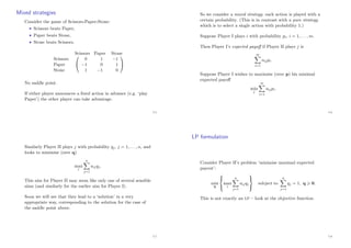
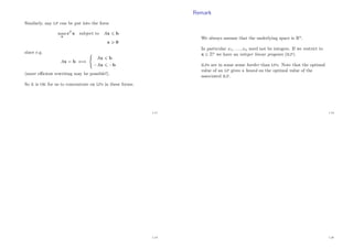
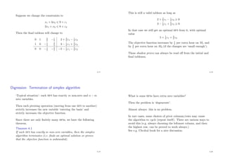
Definition 2.1
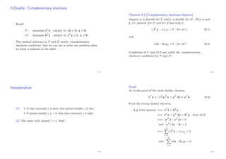
A set S ⊂ Rn is called convex if for all u, v ∈ S and all
λ ∈ (0, 1), we have λu + (1 − λ)v ∈ S.
u
v
convex
v
u
convex
u
v
not convex
That is, a set is convex if all points on the line segment joining
u and v are in S, for all possible line segments.
2.1
For now we will consider LPs in the form
max cT
x subject to Ax = b
x 0.
2.2
Theorem 2.2
The feasible set
S = {x ∈ Rn
: Ax = b, x 0}
is convex.
Proof.
Suppose u, v ∈ S, λ ∈ (0, 1). Let w = λu + (1 − λ)v. Then
Aw = A[λu + (1 − λ)v]
= λAu + (1 − λ)Av
= [λ + (1 − λ)]b
= b
and w λ0 + (1 − λ)0 = 0. So w ∈ S.
2.3
Extreme points
Definition 2.3
A point x in a convex set S is called an extreme point of S if
there are no two distinct points u, v ∈ S, and λ ∈ (0, 1), such
that x = λu + (1 − λ)v.
That is, an extreme point x is not in the interior of any line
segment lying in S.
2.4

7. Theorem 2.4
If an LP has an optimal solution, then it has an optimal
solution at an extreme point of the feasible set.
Proof.
Idea: If the optimum is not extremal, it’s on some line within S
all of which is optimal: go to the end of that line, repeat if
necessary.
Since there exists an optimal solution, there exists an optimal
solution x with a minimal number of non-zero components.
Suppose x is not extremal, so that
x = λu + (1 − λ)v
for some u = v ∈ S, λ ∈ (0, 1).
2.5
Since x is optimal, cT u cT x and cT v cT x.
But also cT x = λcT u + (1 − λ)cT v so in fact cT u = cT v = cT x.
Now consider the line defined by
x(ε) = x + ε(u − v), ε ∈ R.
Then
(a) Ax = Au = Av = b so Ax(ε) = b for all ε,
(b) cT x(ε) = cT x for all ε,
(c) if xi = 0 then ui = vi = 0, which implies x(ε)i = 0 for all ε,
(d) if xi > 0 then x(0)i > 0, and x(ε)i is continuous in ε.
2.6
So we can increase ε from zero, in a positive or a negative
direction as appropriate, until at least one extra component of
x(ε) becomes zero.
This gives an optimal solution with fewer non-zero components
than x.
So x must be extreme.
2.7
Basic solutions
Let ai be the ith column of A, so that
Ax = b ⇐⇒
n
i=1
xiai = b.
Definition 2.5
(1) A solution x of Ax = b is called a basic solution if the
vectors {ai : xi = 0} are linearly independent.
(That is, columns of A corresponding to non-zero variables
xi are linearly independent.)
(2) A basic solution satisfying x 0 is called a basic feasible
solution (BFS).
Note: If A has m rows, then at most m columns can be linearly
independent. So any basic solution x has at least n − m zero
components. More later.
2.8

8. Theorem 2.6
x is an extreme point of
S = {x : Ax = b, x 0}
if and only if x is a BFS.
Proof.
(1) Let x be a BFS. Suppose x = λu + (1 − λ)v for u, v ∈ S,
λ ∈ (0, 1). To show x is extreme we need to show u = v.
Let I = {i : xi > 0}. Then
(a) if i ∈ I then xi = 0, which implies ui = vi = 0.
2.9
(b) Au = Av = b, so A(u − v) = 0
=⇒
n
i=1
(ui − vi)ai = 0
=⇒
i∈I
(ui − vi)ai = 0 since ui = vi = 0 for i ∈ I
which implies ui = vi for i ∈ I since {ai : i ∈ I} are linearly
independent.
Hence u = v, so x is an extreme point.
2.10
(2) Suppose x is not a BFS, i.e. {ai : i ∈ I} are linearly
dependent.
Then there exists u = 0 with ui = 0 for i ∈ I such that
Au = 0.
For small enough ε, x ± εu are feasible, and
x =
1
2
(x + εu) +
1
2
(x − εu)
so x is not extreme.
2.11
Corollary 2.7
If there is an optimal solution, then there is an optimal BFS.
Proof.
This is immediate from Theorems 2.4 and 2.6.
2.12

9. Discussion
Typically we may assume:
• n > m (more variables than constraints),
• A has rank m (its rows are linearly independent; if not,
either we have a contradiction, or redundancy).
Then: x is a basic solution ⇐⇒ there is a set B ⊂ {1, . . . , n}
of size m such that
• xi = 0 if i ∈ B,
• {ai : i ∈ B} are linearly independent.
Proof.
Simple exercise. Take I = {i : xi = 0} and augment it to a
larger linearly independent set B if necessary.
2.13
Then to look for basic solutions:
• choose n − m of the n variables to be 0 (xi = 0 for i ∈ B),
• look at remaining m columns {ai : i ∈ B}.
Are they linearly independent? If so we have an invertible
m × m matrix.
Solve for {xi : i ∈ B} to give i∈B xiai = b.
So also
Ax =
n
i=1
xiai =
n
i∈B
0ai +
n
i∈B
xiai
= b as required.
This way we obtain all basic solutions (at most n
m of them).
2.14
Bad algorithm:
• look through all basic solutions,
• which are feasible?
• what is the value of the objective function?
We can do much better!
Simplex algorithm:
• will move from one BFS to another, improving the value of
the objective function at each step.
2.15 2.16

10. 3 The simplex algorithm (1)
The simplex algorithm works as follows.
1. Start with an initial BFS.
2. Is the current BFS optimal?
3. If YES, stop.
If NO, move to a new and improved BFS, then return to 2.
From Corollary 2.7, it is sufficient to consider only BFSs when
searching for an optimal solution.
3.1
Recall P1, expressed without slack variables:
maximise x1 + x2
subject to x1 + 3x2 9
2x1 + x2 8
x1, x2 0
3.2
x1
x2
x1 + 3x2 = 92x1 + x2 = 8
A
B
E
D F
C
3.3
Rewrite:
x1 +3x2 +x3 = 9 (1)
2x1 + x2 +x4 = 8 (2)
x1 + x2 = f(x) (3)
Put x1, x2 = 0, giving x3 = 9, x4 = 8, f = 0 (we’re at the BFS
x = (0, 0, 9, 8)).
Note: In writing the three equations as (1)–(3) we are
effectively expressing x3, x4, f in terms of x1, x2.
3.4

11. 1. Start at the initial BFS x = (0, 0, 9, 8), vertex A, where f = 0.
2. From (3), increasing x1 or x2 will increase f(x). Let’s
increase x1.
(a) From (1): we can increase x1 to 9, if we decrease x3 to 0.
(b) From (2): we can increase x1 to 4, if we decrease x4 to 0.
The stricter restriction on x1 is (b).
3. So (keeping x2 = 0),
(a) increase x1 to 4, decrease x4 to 0 – using (2), this maintains
equality in (2),
(b) and, using (1), decreasing x3 to 5 maintains equality in (1).
With these changes we move to a new and improved BFS
x = (4, 0, 5, 0), f(x) = 4, vertex D.
3.5
To see if this new BFS is optimal, rewrite (1)–(3) so that
• each non-zero variable appears in exactly one constraint,
• f is in terms of variables which are zero at vertex D.
Alternatively, we want to express x1, x3, f in terms of x2, x4.
How? Add multiples of (2) to the other equations.
3.6
(1) − 1
2 × (2) : 5
2x2 +x3 −1
2x4 = 5 (4)
1
2 × (2) : x1 +1
2x2 +1
2x4 = 4 (5)
(3) − 1
2 × (2) : 1
2x2 −1
2x4 = f − 4 (6)
Now f = 4 + 1
2x2 − 1
2x4.
So we should increase x2 to increase f.
3.7
1 . We are at vertex D, x = (4, 0, 5, 0) and f = 4.
2 . From (6), increasing x2 will increase f (increasing x4 would
decrease f).
(a) From (4): we can increase x2 to 2, if we decrease x3 to 0.
(b) From (5): we can increase x2 to 8, if we decrease x1 to 0.
The stricter restriction on x2 is (a).
3 . So increase x2 to 2, decrease x3 to 0 (x4 stays at 0, and from
(5) x1 decreases to 3).
With these changes we move to the BFS x = (3, 2, 0, 0),
vertex C.
3.8

12. Rewrite (4)–(6) so that they correspond to vertex C:
2
5 × (4) : x2 +2
5x3 −1
5x4 = 2 (7)
(5) − 1
5 × (4) : x1 −1
5x3 +3
5x4 = 3 (8)
(6) − 1
5 × (4) : −1
5x3 −2
5x4 = f − 5 (9)
1 . We are at vertex C, x = (3, 2, 0, 0) and f = 5.
2 . We have deduced f = 5 − 1
5x3 − 2
5x4 5.
So x3 = x4 = 0 is the best we can do!
In that case we can read off x1 = 3 and x2 = 2.
So x = (3, 2, 0, 0), which has f = 5, is optimal.
3.9
Summary
At each stage:
• B = ‘basic variables’,
• we express xi, i ∈ B and f in terms of xi, i ∈ B,
• setting xi = 0, i ∈ B, we can read off f and xi, i ∈ B (gives
a BFS!).
At each update:
• look at f in terms of xi, i ∈ B,
• which xi, i ∈ B, would we like to increase?
• if none, STOP!
• otherwise, choose one and increase it as much as possible,
i.e. until one variable xi, i ∈ B, becomes 0.
3.10
Summary continued
So
• one new variable enters B (becomes non-zero, becomes
basic),
• another one leaves B (becomes 0, becomes non-basic).
This gives a new BFS.
We update our expressions to correspond to the new B.
3.11
Simplex algorithm
We can write equations
x1 +3x2 +x3 = 9 (1)
2x1 + x2 +x4 = 8 (2)
x1 + x2 = f − 0 (3)
as a ‘tableau’
x1 x2 x3 x4
1 3 1 0 9 ρ1
2 1 0 1 8 ρ2
1 1 0 0 0 ρ3
This initial tableau represents the BFS x = (0, 0, 9, 8) at which
f = 0.
Note the identity matrix in the x3, x4 columns (first two rows),
and the zeros in the bottom row below it.
3.12

13. The tableau
At a given stage, the tableau has the form
(aij) b
cT f
which means
Ax = b
f(x) = cT
x − f
We start from A = A, b = b, c = c and f = 0.
Updating the tableau is called pivoting.
3.13
To update (‘pivot’)
1. Choose a pivot column
Choose a j such that cj > 0 (corresponds to variable xj = 0
that we want to increase).
Here we can take j = 1 .
2. Choose a pivot row
Among the i’s with aij > 0, choose i to minimize bi/aij
(strictest limit on how much we can increase xj).
Here take i = 2 since 8/2 < 9/1.
3.14
3. Do row operations so that column j gets a 1 in row i and 0s
elsewhere:
• multiply row i by
1
aij
,
• for i = i,
add −
ai j
aij
× (row i) to row i ,
• add −
cj
aij
× (row i) to objective function row.
3.15
In our example we pivot on j = 1, i = 2. The updated tableau is
x1 x2 x3 x4
0 5
2 1 −1
2 5 ρ1 = ρ1 − ρ2
1 1
2 0 1
2 4 ρ2 = 1
2ρ2
0 1
2 0 −1
2 −4 ρ3 = ρ3 − ρ2
which means
5
2x2 +x3 −1
2x4 = 5
x1 +1
2x2 +1
2x4 = 4
1
2x2 −1
2x4 = f − 4
‘non-basic variables’ x2, x4 are 0, x = (4, 0, 5, 0).
Note the identity matrix inside (aij) telling us this.
3.16

14. Next pivot: column 2, row 1 since
5
5/2
<
4
1/2
.
x1 x2 x3 x4
0 1 2
5 −1
5 2 ρ1 = 2
5ρ1
1 0 −1
5
3
5 3 ρ2 = ρ2 − 1
2ρ1
0 0 −1
5 −2
5 −5 ρ3 = ρ3 − 1
2ρ1
Now we have only non-positive entries in the bottom row: STOP.
x = (3, 2, 0, 0), f(x) = 5 optimal.
3.17
Geometric picture for P1
x1
x2
x1 + 3x2 = 92x1 + x2 = 8
A
B
E
D F
C
3.18
x1 x2 x3 x4
A 0 0 9 8
B 4 0 5 0
C 3 2 0 0
D 0 3 0 5
A, B, C, D are BFSs. E, F are basic solutions but not feasible.
Simplex algorithm: A → D → C (or A → B → C is we choose a
different column for the first pivot).
Higher-dimensional problems less trivial!
3.19
Comments on simplex tableaux
• We always find an m × m identity matrix embedded in
(aij), in the columns corresponding to basic variables xi,
i ∈ B,
• in the objective function row (bottom row) we find zeros in
these columns.
Hence f and xi, i ∈ B, are all written in terms of xi, i ∈ B.
Since we set xi = 0 for i ∈ B, it’s then trivial to read off f and
xi, i ∈ B.
3.20

15. Comments on simplex algorithm
• Choosing a pivot column
We may choose any j such that cj > 0. In general, there is
no way to tell which such j result in fewest pivot steps.
• Choosing a pivot row
Having chosen pivot column j (which variable xj to
increase), we look for rows with aij > 0.
If aij 0, constraint i places no restriction on the increase
of xj.
If aij 0 for all i, xj can be increased without limit: the
objective function is unbounded.
Otherwise, the most stringent limit comes from the i that
minimises bi/aij.
3.21 3.22
3.23 3.24

16. 4 The simplex algorithm (2)
Two issues to consider:
• can we always find a BFS from which to start the simplex
algorithm?
• does the simplex algorithm always terminate, i.e. find an
optimal BFS or prove the problem is unbounded?
4.1
Initialisation
To start the simplex algorithm, we need to start from a BFS,
with basic variables xi, i ∈ B, written in terms of non-basic
variables xi, i ∈ B.
If A already contains Im as an m × m submatrix, this is usually
easy!
This always happens if b 0 and A is created by adding slack
variables to make inequalities into equalities.
4.2
Suppose the constraints are
Ax b, x 0
where b 0. Then an initial BFS is immediate: introducing
slack variables z = (z1, . . . , zm),
Ax + z = b, x, z 0
so the initial tableau is
x1 · · · xn z1 · · · zm
A Im b
cT 0T 0
and an initial BFS is x
z = 0
b .
4.3
Example
max 6x1 + x2 + x3
s.t. 9x1 + x2 + x3 18
24x1 + x2 + 4x3 42
12x1 + 3x2 + 4x3 96
x1, x2, x3 0.
Add slack variables:
9x1 + x2 + x3 + w1 = 18
24x1 + x2 + 4x3 + w2 = 42
12x1 + 3x2 + 4x3 + w3 = 96
4.4

17. Solve by simplex
9 1 1 1 0 0 18
24 1 4 0 1 0 42
12 3 4 0 0 1 96
6 1 1 0 0 0 0
This initial tableau is already in the form we need.
9 1 1 1 0 0 18 ρ1 = ρ1
15 0 3 −1 1 0 24 ρ2 = ρ2 − ρ1
−15 0 1 −3 0 1 42 ρ3 = ρ3 − 3ρ1
−3 0 0 −1 0 0 −18 ρ4 = ρ4 − ρ1
This solution is optimal: x2 = 18, x1 = 0, x3 = 0, f = 18.
4.5
What if A doesn’t have this form?
In general we can write the constraints as
Ax = b, x 0 (4.1)
where b 0 (if necessary, multiply rows by −1 to get b 0).
If there is no obvious initial BFS and we need to find one, we
can introduce artificial variables w1, . . . , wm and solve the LP
problem
min
x,w
m
i=1
wi
subject to Ax + w = b
x, w 0.
(4.2)
4.6
Two cases arise:
(1) if (4.1) has a feasible solution, then (4.2) has optimal
value 0 with w = 0.
(2) if (4.1) has no feasible solution, then the optimal value of
(4.2) is > 0.
We can apply the simplex algorithm to determine whether it’s
case (1) or (2).
• In case (2), give up.
• In case (1), the optimal BFS for (4.2) with wi ≡ 0 gives a
BFS for (4.1)!
This leads us to the two-phase simplex algorithm.
4.7
Two-phase simplex algorithm
Example:
maximize 3x1 + x3
subject to x1 + 2x2 + x3 = 30
x1 − 2x2 + 2x3 = 18
x 0
With artificial variables:
minimize w1 + w2
subject to x1 + 2x2 + x3 + w1 = 30
x1 − 2x2 + 2x3 + w2 = 18
x, w 0.
4.8

18. Note: To minimise w1 + w2, we can maximise −w1 − w2. So
start from the simple tableau
x1 x2 x3 w1 w2
1 2 1 1 0 30
1 −2 2 0 1 18
0 0 0 −1 −1 0
The objective function row should be expressed in terms of
non-basic variables (the entries under the ‘identity matrix’
should be 0).
4.9
So start by adding row 1 + row 2 to objective row:
x1 x2 x3 w1 w2
1 2 1 1 0 30
1 −2 2 0 1 18
2 0 3 0 0 48
Now start with simplex – pivot on a23:
x1 x2 x3 w1 w2
1
2 3 0 1 −1
2 21
1
2 −1 1 0 1
2 9
1
2 3 0 0 −3
2 21
4.10
Pivot on a12:
x1 x2 x3 w1 w2
1
6 1 0 1
3 −1
6 7
2
3 0 1 1
3
1
3 16
0 0 0 −1 −1 0
So we have found a point with −w1 − w2 = 0, i.e. w = 0.
Phase I is finished. BFS of the original problem is x = (0, 7, 16).
4.11
Deleting the w columns and replacing the objective row by the
original objective function 3x1 + x3:
x1 x2 x3
1
6 1 0 7
2
3 0 1 16
3 0 1 0
Again we want zeros below the identity matrix – subtract row 2
from row 3:
x1 x2 x3
1
6 1 0 7
2
3 0 1 16
7
3 0 0 −16
Now do simplex.
4.12

19. Pivot on a21:
x1 x2 x3
0 1 −1
4 3
1 0 3
2 24
0 0 −7
2 −72
Done! Maximum at x1 = 24, x2 = 3, x3 = 0, f = 72.
4.13
Shadow prices
Recall P1:
max x1 + x2
s.t. x1 + 3x2 9
2x1 + x2 8
x1, x2 0
4.14
We had initial tableau
1 3 1 0 9 ρ1
2 1 0 1 8 ρ2
1 1 0 0 0 ρ3
and final tableau
0 1 2
5 −1
5 2 ρ1
1 0 −1
5
3
5 3 ρ2
0 0 −1
5 −2
5 −5 ρ3
From the mechanics of the simplex algorithm:
• ρ1, ρ2 are created by taking linear combinations of ρ1, ρ2
• ρ3 is ρ3 − (a linear combination of ρ1, ρ2).
4.15
Directly from the tableaux (look at columns 3 and 4):
ρ1 = 2
5ρ1 − 1
5ρ2
ρ2 = −1
5ρ1 + 3
5ρ2
ρ3 = ρ3 − 1
5ρ1 − 2
5ρ2
4.16

20. Suppose we change the constraints to
x1 + 3x2 9 + ε1
2x1 + x2 8 + ε2.
Then the final tableau will change to
0 1 2
5 −1
5 2 + 2
5ε1 − 1
5ε2
1 0 −1
5
3
5 3 − 1
5ε1 + 3
5ε2
0 0 −1
5 −2
5 −5 − 1
5ε1 − 2
5ε2
4.17
This is still a valid tableau as long as
2 + 2
5ε1 − 1
5ε2 0
3 − 1
5ε1 + 3
5ε2 0.
In that case we still get an optimal BFS from it, with optimal
value
5 + 1
5ε1 + 2
5ε2.
The objective function increases by 1
5 per extra hour on M1 and
by 2
5 per extra hour on M2 (if the changes are ‘small enough’).
These shadow prices can always be read off from the initial and
final tableaux.
4.18
Digression: Termination of simplex algorithm
‘Typical situation’: each BFS has exactly m non-zero and n − m
zero variables.
Then each pivoting operation (moving from one BFS to another)
strictly increases the new variable ‘entering the basis’ and
strictly increases the objective function.
Since there are only finitely many BFSs, we have the following
theorem.
Theorem 4.1
If each BFS has exactly m non-zero variables, then the simplex
algorithm terminates (i.e. finds an optimal solution or proves
that the objective function is unbounded).
4.19
What is some BFSs have extra zero variables?
Then the problem is ‘degenerate’.
Almost always: this is no problem.
In rare cases, some choices of pivot columns/rows may cause
the algorithm to cycle (repeat itself). There are various ways to
avoid this (e.g. always choosing the leftmost column, and then
the highest row, can be proved to work always.)
See e.g. Chv´atal book for a nice discussion.
4.20

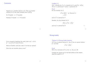
21. 5 Duality: Introduction
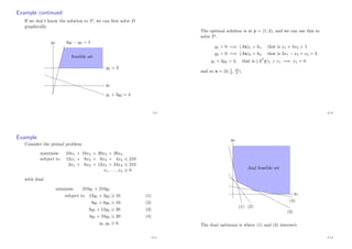
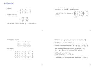
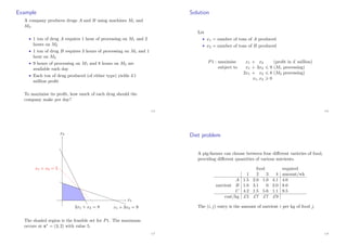
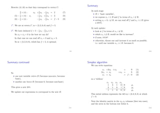
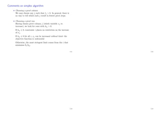
Recall P1:
maximise x1 + x2
subject to x1 + 3x2 9 (5.1)
2x1 + x2 8 (5.2)
x1, x2 0.
‘Obvious’ bounds on f(x) = x1 + x2:
x1 + x2 x1 + 3x2 9 from (5.1)
x1 + x2 2x1 + x2 8 from (5.2).
By combining the constraints we can improve the bound, e.g.
1
3[(5.1) + (5.2)]:
x1 + x2 x1 + 4
3x2
17
3 .
5.1
More systematically?
For y1, y2 0, consider y1 × (5.1) + y2 × (5.2). We obtain
(y1 + 2y2)x1 + (3y1 + y2)x2 9y1 + 8y2
Since we want an upper bound for x1 + x2, we need
coefficients 1:
y1 + 2y2 1
3y1 + y2 1.
How to get the best bound by this method?
D1 : minimise 9y1 + 8y2
subject to y1 + 2y2 1
3y1 + y2 1
y1, y2 0.
P1 = ‘primal problem’, D1 = ‘dual of P1’.
5.2
Duality: General
In general, given a primal problem
P : maximise cT
x subject to Ax b, x 0
the dual of P is defined by
D : minimise bT
y subject to AT
y c, y 0.
Exercise
The dual of the dual is the primal.
5.3
Weak duality
Theorem 5.1 (Weak duality theorem)
If x is feasible for P, and y is feasible for D, then
cT
x bT
y.
Proof.
Since x 0 and AT y c: cT x (AT y)T x = yT Ax.
Since y 0 and Ax b: yT Ax yT b = bT y.
Hence cT x yT Ax bT y.
5.4

22. Comments
Suppose y is a feasible solution to D. Then any feasible
solution x to P has value bounded above by bT y.
So D feasible =⇒ P bounded.
Similarly P feasible =⇒ D bounded.
5.5
Corollary 5.2
If x∗ is feasible for P, y∗ is feasible for D, and cT x∗ = bT y∗,
then x∗ is optimal for P and y∗ is optimal for D.
Proof.
For all x feasible for P,
cT
x bT
y∗
by Theorem 5.1
= cT
x∗
and so x∗ is optimal for P.
Similarly, for all y feasible for D,
bT
y cT
x∗
= bT
y∗
and so y∗ is optimal for D.
5.6
As an example of applying this result, look at x∗ = (3, 2),
y∗ = (1
5, 2
5) for P1 and D1 above.
Both are feasible, both have value 5. So both are optimal.
Does this nice situation always occur?
5.7
Strong duality
Theorem 5.3 (Strong duality theorem)
If P has an optimal solution x∗, then D has an optimal solution
y∗ such that
cT
x∗
= bT
y∗
.
Proof.
Write the constraints of P as Ax + z = b, x, z 0.
Consider the bottom row in the final tableau of the simplex
algorithm applied to P.
5.8

23. x-columns z-columns
c∗
1 · · · c∗
n −y∗
1 · · · −y∗
m −f∗
Here f∗ is the optimal value of cT x,
c∗
j 0 for all j (5.3)
−y∗
i 0 for all i (5.4)
and the bottom row tells us that
cT
x − f∗
= c∗T
x − y∗T
z.
5.9
Thus
cT
x = f∗
+ c∗T
x − y∗T
z
= f∗
+ c∗T
x − y∗T
(b − Ax)
= f∗
− bT
y∗
+ (c∗T
+ y∗T
A)x.
This is true for all x, so
f∗
= bT
y∗
(5.5)
c = AT
y∗
+ c∗
.
From (5.3) c∗ 0, hence
AT
y∗
c. (5.6)
5.10
So (5.4) and (5.6) show that y∗ is feasible for D.
And (5.5) shows that the objective function of D at y∗ is
bT y∗ = f∗ = optimal value of P.
So from the weak duality theorem (Theorem 5.1), y∗ is optimal
for D.
5.11
Comments
Note:
• the coefficients y∗ from the bottom row in the columns
corresponding to slack variables give us the optimal
solution to D,
• comparing with the shadow prices discussion: these
optimal dual variables are the shadow prices!
5.12

24. Example
It is possible that neither P nor D has a feasible solution:
consider the problem
maximise 2x1 − x2
subject to x1 − x2 1
− x1 + x2 −2
x1, x2 0.
5.13
Example
Consider the problem
maximise 2x1 + 4x2 + x3 + x4
subject to x1 + 3x2 + x4 4
2x1 + x2 3
x1 + 4x3 + x4 3
x1, . . . , x4 0
5.14
The final tableau is
x1 x2 x3 x4 x5 x6 x7
0 1 0 2
5
2
5 · · 1
1 0 0 −1
5 −1
5 · · 1
0 0 1 3
10
1
20 · · 1
2
0 0 0 −1
2 −5
4 −1
4 −1
4 −13
2
(1) By the proof of Theorem 5.3, y∗ = (5
4, 1
4, 1
4) is optimal for
the dual.
5.15
(2) Suppose the RHSs of the original constraints become 4 + ε1,
3 + ε2, 3 + ε3. Then the objective function becomes
13
2 + 5
4ε1 + 1
4ε2 + 1
4ε3.
If the original RHSs of 4, 3, 3 correspond to the amount of
raw material i available, then ‘the most you’d be prepared
to pay per additional unit of raw material i’ is y∗
i (with y∗
as in (1)).
5.16

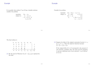
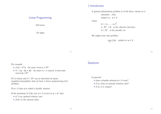
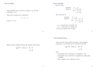
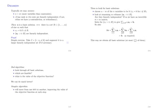
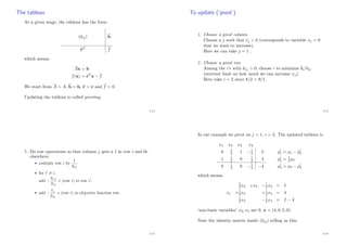
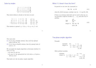
25. (3) Suppose raw material 1 is available at a price < 5
4 per unit.
How much should you buy? With ε1 > 0, ε2 = ε3 = 0, the
final tableau would be
1 + 2
5ε1
· · · 1 − 1
5ε1
1
2 + 1
20ε1
For this tableau to represent a BFS, the three entries in the
final column must be 0, giving ε1 5. So we should buy
5 additional units of raw material 1.
5.17
(4) The optimal solution x∗ = (1, 1, 1
2, 0) is unique as the
entries in the bottom row corresponding to non-basic
variables (i.e. the −1
2, −5
4, −1
4, −1
4) are < 0.
(5) If say the −5
4 was zero, we could pivot in that column
(observe that there would somewhere to pivot) to get a
second optimal BFS x∗∗. Then λx∗ + (1 − λ)x∗∗ would be
optimal for all λ ∈ [0, 1].
5.18
5.19 5.20

26. 6 Duality: Complementary slackness
Recall
P : maximise cT
x subject to Ax b, x 0,
D : minimise bT
y subject to AT
y c, y 0.
The optimal solutions to P and D satisfy ‘complementary
slackness conditions’ that we can use to solve one problem when
we know a solution of the other.
6.1
Theorem 6.1 (Complementary slackness theorem)
Suppose x is feasible for P and y is feasible for D. Then x and
y are optimal (for P and D) if and only if
(AT
y − c)jxj = 0 for all j (6.1)
and
(Ax − b)iyi = 0 for all i. (6.2)
Conditions (6.1) and (6.2) are called the complementary
slackness conditions for P and D.
6.2
Interpretation
(1) • If dual constraint j is slack, then primal variable j is zero.
• If primal variable j is > 0, then dual constraint j is tight.
(2) The same with ‘primal’ ←→ ‘dual’.
6.3
Proof.
As in the proof of the weak duality theorem,
cT
x (AT
y)T
x = yT
Ax yT
b. (6.3)
From the strong duality theorem,
x, y both optimal ⇐⇒ cT
x = bT
y
⇐⇒ cT
x = yT
Ax = bT
y from (6.3)
⇐⇒ (yT
A − cT
)x = 0
and yT
(Ax − b) = 0
⇐⇒
n
j=1
(AT
y − c)jxj = 0
and
m
i=1
(Ax − b)iyi = 0.
6.4

27. But AT y c and x 0, so n
j=1(AT y − c)jxj is a sum of
non-negative terms.
Also, Ax b and y 0, so m
i=1(Ax − b)iyi is a sum of
non-positive terms.
Hence n
j=1(AT y − c)jxj = 0 and m
i=1(Ax − b)iyi = 0 is
equivalent to (6.1) and (6.2).
6.5
Comments
What’s the use of complementary slackness?
Among other things, given an optimal solution of P (or D), it
makes finding an optimal solution of D (or P) very easy,
because we know which the non-zero variables can be and which
constraints must be tight.
Sometimes one of P and D is much easier to solve than the
other, e.g. with 2 variables, 5 constraints, we can solve
graphically, but 5 variables and 2 constraints is not so easy.
6.6
Example
Consider P and D with
A =
1 4 0
3 −1 1
, b =
1
3
, c =


4
1
3

 .
Is x = (0, 1
4, 13
4 ) optimal? It is feasible. If it is optimal, then
x2 > 0 =⇒ (AT
y)2 = c2, that is 4y1 − y2 = 1
x3 > 0 =⇒ (AT
y)3 = c3, that is 0y1 + y2 = 3
which gives y = (y1, y2) = (1, 3).
The remaining dual constraint y1 + 3y2 4 is also satisfied, so
y = (1, 3) is feasible for D.
6.7
So x = (0, 1
4, 13
4 ) and y = (1, 3) are feasible and satisfy
complementary slackness, therefore they are optimal by
Theorem 6.1.
Alternatively, we could note that this x and y are feasible and
cT x = 10 = bT y, so they are optimal by Corollary 5.2.
6.8

28. Example continued
If we don’t know the solution to P, we can first solve D
graphically.
feasible set
y1
y2
y2 = 3
y1 + 3y2 = 4
4y1 − y2 = 1
6.9
The optimal solution is at y = (1, 3), and we can use this to
solve P:
y1 > 0 =⇒ (Ax)1 = b1, that is x1 + 4x2 = 1
y2 > 0 =⇒ (Ax)2 = b2, that is 3x1 − x2 + x3 = 3
y1 + 3y2 > 4, that is (AT
y)1 > c1 =⇒ x1 = 0
and so x = (0, 1
4, 13
4 ).
6.10
Example
Consider the primal problem
maximise 10x1 + 10x2 + 20x3 + 20x4
subject to 12x1 + 8x2 + 6x3 + 4x4 210
3x1 + 6x2 + 12x3 + 24x4 210
x1, . . . , x4 0
with dual
minimise 210y1 + 210y2
subject to 13y1 + 3y2 10 (1)
8y1 + 6y2 10 (2)
6y1 + 12y2 20 (3)
4y1 + 24y2 20 (4)
y1, y2 0.
6.11
dual feasible set
y1
y2
(1) (2)
(3)
(4)
The dual optimum is where (1) and (3) intersect.
6.12

29. Since the second and fourth dual constraints are slack at the
optimum, the optimal x has x2 = x4 = 0.
Also, since y1, y2 > 0 at the optimum,
12x1 + 6x3 = 210
3x1 + 12x3 = 210
=⇒ x1 = 10, x3 = 15.
Hence the optimal x is (10, 0, 15, 0).
6.13
Example continued
Suppose the second 210 is replaced by 421.
The new dual optimum is where (3) and (4) intersect, at which
point the first two constraints are slack, so x1 = x2 = 0.
Also, since y1, y2 > 0 at the new optimum,
6x3 + 4x4 = 210
12x3 + 24x4 = 421
=⇒ x3 = 35 − 1
24, x4 = 1
16.
So the new optimum is at x = (0, 0, 35 − 1
24, 1
16).
6.14
6.15 6.16

30. 7 Two-player zero-sum games (1)
We consider games that are ‘zero-sum’ in the sense that one
player wins what the other loses.
Each player has a choice of actions (the choices may be different
for each player).
Players move simultaneously.
7.1
Payoff matrix
There is a payoff matrix A = (aij):
Player II plays j
1
Player I plays i 2
3


1 2 3 4
−5 3 1 20
5 5 4 6
−4 6 0 −5


If Player I plays i and Player II plays j, then Player I wins aij
from Player II.
The game is defined by the payoff matrix.
Note that our convention is that I wins aij from II, so aij > 0 is
good for Player I = row player.
7.2
What’s the ‘worst that can happen’ to Player I if Player I
chooses row 1? row 2? row 3? (We look at the smallest entry in
the appropriate row.)
What’s the ‘worst that can happen’ to Player II if Player II
chooses a particular column? (We look at the largest entry in
that column.)
The matrix above has a special property.
Entry a23 = 4 is both
• the smallest entry in row 2
• the largest entry in column 3
(2, 3) is a ‘saddle point’ of A.
7.3
Thus:
• Player I can guarantee to win at least 4 by choosing row 2.
• Player II can guarantee to lose at most 4 by choosing
column 3.
• The above is still true if either player announces their
strategy in advance.
Hence the game is ‘solved’ and it has ‘value’ 4.
7.4

31. Mixed strategies
Consider the game of Scissors-Paper-Stone:
• Scissors beats Paper,
• Paper beats Stone,
• Stone beats Scissors.
Scissors Paper Stone
Scissors
Paper
Stone


0
−1
1
1
0
−1
−1
1
0


No saddle point.
If either player announces a fixed action in advance (e.g. ‘play
Paper’) the other player can take advantage.
7.5
So we consider a mixed strategy: each action is played with a
certain probability. (This is in contrast with a pure strategy
which is to select a single action with probability 1.)
Suppose Player I plays i with probability pi, i = 1, . . . , m.
Then Player I’s expected payoff if Player II plays j is
m
i=1
aijpi.
Suppose Player I wishes to maximise (over p) his minimal
expected payoff
min
j
m
i=1
aijpi.
7.6
Similarly Player II plays j with probability qj, j = 1, . . . , n, and
looks to minimise (over q)
max
i
n
j=1
aijqj.
This aim for Player II may seem like only one of several sensible
aims (and similarly for the earlier aim for Player I).
Soon we will see that they lead to a ‘solution’ in a very
appropriate way, corresponding to the solution for the case of
the saddle point above.
7.7
LP formulation
Consider Player II’s problem ‘minimise maximal expected
payout’:
min
q



max
i
n
j=1
aijqj



subject to
n
j=1
qj = 1, q 0.
This is not exactly an LP – look at the objective function.
7.8

32. Equivalent formulation
An equivalent formulation is:
min
q,v
v subject to
m
j=1
aijqj v for i = 1, . . . , m
n
j=1
qj = 1
q 0.
since v, on being minimised, will decrease until it takes the
value of maxi
n
j=1 aijqj.
This is an LP but not exactly in a useful form for our methods.
We will transform it!
7.9
First add a constant k to each aij so that aij > 0 for all i, j.
This doesn’t change the nature of the game, but guarantees
v > 0.
So WLOG, assume aij > 0 for all i, j.
Now change variables to xj = qj/v. The problem becomes:
min
x,v
v subject to
m
j=1
aijxj 1 for i = 1, . . . , m
n
j=1
xj = 1/v
x 0.
7.10
This transformed problem for Player II is equivalent to
P : max
x
n
j=1
xj subject to Ax 1, x 0
which is now in our ‘standard form’. (1 denotes a vector of 1s.)
7.11
Doing the same transformations for Player I’s problem
max
p
min
j
m
i=1
aijpi subject to
m
i=1
pi = 1, p 0
turns into
D : min
y
m
i=1
yi subject to AT
y 1, y 0.
(Check: on problem sheet.)
P and D are dual and hence have the same optimal value.
7.12

33. Conclusion
Let x∗, y∗ be optimal for P, D. Then:
• Player I can guarantee an expected gain of at least
v = 1/ m
i=1 y∗
i , by following strategy p = vy∗.
• Player II can guarantee an expected loss of at most
v = 1/ n
j=1 x∗
j , by following strategy q = vx∗.
• The above is still true if a player announces his strategy in
advance.
So the game is ‘solved’ as in the saddle point case (this was just
a special case where the strategies were pure).
v is the value of the game (the amount that Player I should
‘fairly’ pay to Player II for the chance to play the game).
7.13 7.14
7.15 7.16

34. 8 Two-player zero-sum games (2)
Some games are easy to solve without the LP formulation, e.g.
A =
−2 2
4 −3
Suppose Player I chooses row 1 with probability p, row 2 with
probability 1 − p. The he should maximise
min(−2p + 4(1 − p), 2p − 3(1 − p))
= min(4 − 6p, 5p − 3)
8.1
x1
x2
4 − 6p
5p − 3
1
8.2
So the min is maximised when
4 − 6p = 5p − 3
which occurs when p = 7
11.
And then v = 35
11 − 3 = 2
11.
(We could go on to find Player II’s optimal strategy too.)
8.3
A useful trick: dominated actions
Consider 

4 2 2
1 3 4
3 0 5

 .
Player II should never play column 3, since column 2 is always
at least as good as column 3 (column 2 ‘dominates’ column 3.)
So we reduce to 

4 2
1 3
3 0


Now Player I will never play row 3 since row 1 is always better,
so
4 2
1 3
has the same value (and optimal strategies) as A.
8.4

35. Final example
Consider
A =


−1 0 1
1 −1 0
−1 3 −1
,


add 1 to each entry
˜A =


0 1 2
2 0 1
0 4 0

 .
This has value > 0 (e.g. strategy (1
3, 1
3, 1
3) for Player I).
8.5
Solve the LP for Player II’s optimal strategy:
max
x1,x2,x3
x1 + x2 + x3 subject to


0 1 2
2 0 1
0 4 0




x1
x2
x3




1
1
1


x 0.
8.6
Initial simplex tableau:
0 1 2 1 0 0 1
2 0 1 0 1 0 1
0 4 0 0 0 1 1
1 1 1 0 0 0 0
final tableau:
0 0 1 1
2 0 −1
8
3
8
1 0 0 −1
4
1
2
1
16
5
16
0 1 0 0 0 1
4
1
4
0 0 0 −1
4 −1
2 − 3
16 −15
16
8.7
Optimum: x1 = 5
16, x2 = 1
4, x3 = 3
8, and x1 + x2 + x3 = 15
16.
So value v = 1/(x1 + x2 + x3) = 16
15.
Player II’s optimal strategy: q = vx = 16
15( 5
16, 1
4, 3
8) = (1
3, 4
15, 2
5).
Dual problem for Player I’s strategy has solution y1 = 1
4,
y2 = 1
2, y3 = 3
16 (from bottom row of final tableau).
So Player I’s optmal strategy:
p = vy = 16
15(1
4, 1
2, 3
16) = ( 4
15, 8
15, 3
15).
˜A has value 16
15, so the original game A has value 16
15 − 1 = 1
15.
8.8