The document provides information on applying Bernoulli's equation and the conservation of mass and energy principles to solve fluid mechanics problems involving pipe flow. It discusses key concepts like:
- Bernoulli's equation relating pressure, velocity, and height.
- How to derive and apply the continuity equation to relate flow rate, velocity, and pipe cross-sectional area.
- The conservation of energy principle and different forms of energy (pressure, potential, kinetic).
- How to set up and solve example problems involving pipe flow and components like nozzles, valves, and changes in pipe diameter or elevation using Bernoulli's equation and accounting for friction losses.
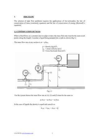
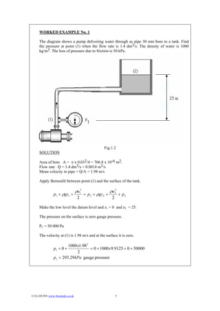
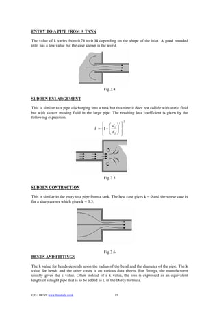
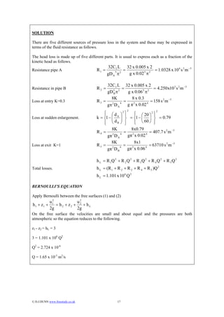
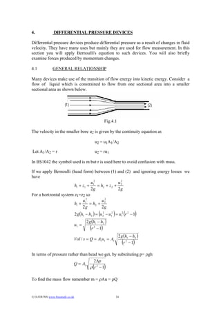
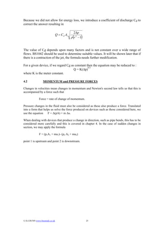
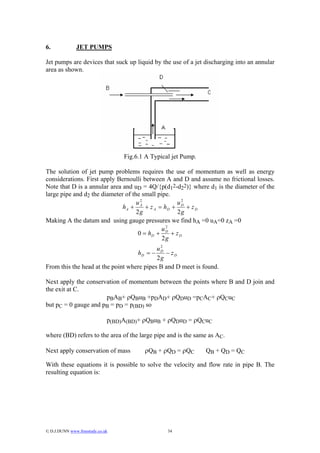
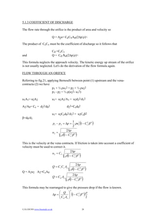
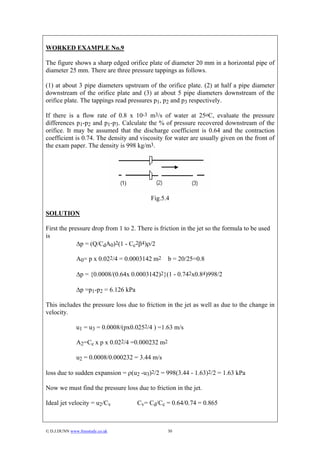
![WORKED EXAMPLE 8
A pipe carrying water experiences a sudden reduction in area as shown. The area at point (1) is
0.002 m2 and at point (2) it is 0.001 m2. The pressure at point (2) is 500 kPa and the velocity is 8
m/s. The loss coefficient K is 0.4. The density of water is 1000 kg/m3. Calculate the following.
i. The mass flow rate.
ii. The pressure at point (1)
iii. The force acting on the section.
Fig.4.2
SOLUTION
u1 = u2A2/A1 = (8 x 0.001)/0.002 = 4 m/s
m = ρA1u1 = 1000 x 0.002 x 4 = 8 kg/s.
Q = A1u1 = 0.002 x 4 = 0.008 m3/s
Pressure loss at contraction = ½ ρku12 = ½ x 1000 x 0.4 x 42 = 3200 Pa
Apply Bernoulli between (1) and (2)
ρu 1
2
ρu 2
p1 + = p2 + 2 + pL
2 2
2
1000 x 4 1000 x 8 2
p1 + = 500 x 10 +
3
+ 3200
2 2
p1 = 527.2 kPa
F = (p1A1 + mu1)- (p2 A2 + mu2)
F = [(527.2 x 103 x 0.002) + (8 x 4)] – [500 x 103 x 0.001) + (8 x 8)]
F = 1054.4 +32 – 500 – 64
F = 522.4 N
© D.J.DUNN www.freestudy.co.uk 26](https://image.slidesharecdn.com/t2203-120217101242-phpapp01/85/T2203-26-320.jpg)
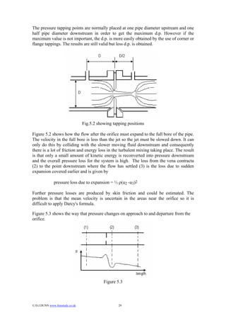
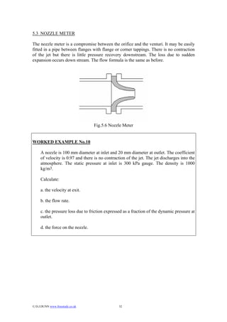
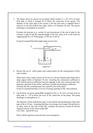
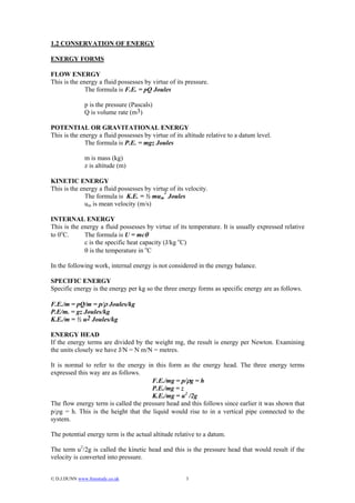
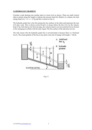
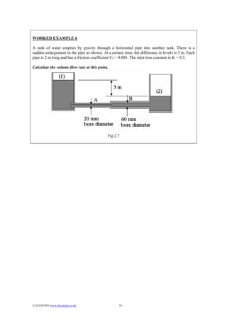
![SOLUTION
The velocity at exit when the inlet velocity is not negligible is
Q = A1Cd[(2∆p/ρ)/(r2 - 1)]0.5
r = A1/A2 = d12/d22 = (100/20)2 = 25
Cd = Cv Cc = 0.97 x 1 = 0.97
A1 = (p x 0.12)/4 = 0.00785 m2
hence Q = 0.97x 0.00785 [(2 x 300 x 103/1000)/(252 - 1)]0.5
Q = 0.00747 m3/s
The velocity at inlet = Q/A1 = 0.00747/0.00785 = 0.951 m/s
The velocity at outlet = Q/A2 = 0.00747 x 4/(p x 0.022)= 23.8 m/s
The dynamic pressure of the jet is ρu22/2 = 1000 x 23.8 2/2 = 282.7 kPa.
Applying Bernoulli between the inlet (1) and outlet (2) using the pressure form we
have
p1 - p2 = ρu22/2 - ρu12/2 + pressure loss to friction
3 x 105 = (1000/2)(23.82 - 0.9512) + pressure loss
3 x 105 = 2.827 x 10⁵ + pressure loss
pressure loss = 17.3 kPa
Expressed as a fraction of the dynamic pressure of the jet this is 17.3/ 282.7 or
6.1%.
The force exerted on the water is given by
F = p1A1 + - p2 A2 + mu1 - mu2
We must use gauge pressures to solve this problem because the atmosphere acts on
the outer surface of the nozzle. The mass flow is 7.47 kg/s.
F = 300 x 103 x 0.00785 - 0 + 7.47(0.951 - 23.8) = 2.18 kN
The figure is positive which indicates the force is accelerating the water out of the
nozzle. The force on the nozzle is the reaction to this and is opposite in direction.
Think of a fireman's hose. The force on the nozzle pushes it away from the water
like a rocket. The force to accelerate the water must be supplied by those holding it.
© D.J.DUNN www.freestudy.co.uk 33](https://image.slidesharecdn.com/t2203-120217101242-phpapp01/85/T2203-33-320.jpg)