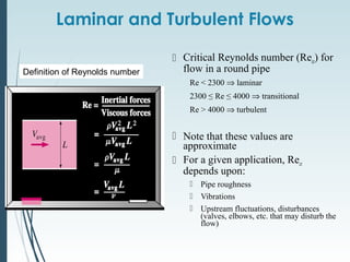
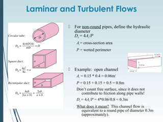
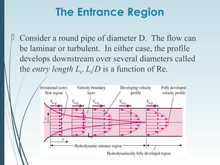
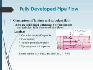
This document discusses laminar and turbulent flow in pipes. It defines the critical Reynolds number that distinguishes between the two flow regimes. For non-circular pipes, it introduces the hydraulic diameter to characterize the pipe geometry. The document then covers topics such as the developing flow region, fully developed flow profiles and pressure drop, the friction factor, minor losses, pipe networks, and pump selection.

1. FLOW IN PIPES

2. Laminar and Turbulent Flows

3. Laminar and Turbulent Flows
 Critical Reynolds number (Recr) for
flow in a round pipe
Re < 2300 ⇒ laminar
2300 ≤ Re ≤ 4000 ⇒ transitional
Re > 4000 ⇒ turbulent
 Note that these values are
approximate
 For a given application, Recr
depends upon:
 Pipe roughness
 Vibrations
 Upstream fluctuations, disturbances
(valves, elbows, etc. that may disturb the
flow)
Definition of Reynolds number

4. Laminar and Turbulent Flows
 For non-round pipes, define the hydraulic
diameter
Dh = 4Ac/P
Ac= cross-section area
P = wetted perimeter
 Example: open channel
Ac = 0.15 * 0.4 = 0.06m2
P = 0.15 + 0.15 + 0.5 = 0.8m
Don’t count free surface, since it does not
contribute to friction along pipe walls!
Dh = 4Ac/P = 4*0.06/0.8 = 0.3m
What does it mean? This channel flow is
equivalent to a round pipe of diameter 0.3m
(approximately).

5. The Entrance Region
 Consider a round pipe of diameter D. The flow can
be laminar or turbulent. In either case, the profile
develops downstream over several diameters called
the entry length Lh. Lh/D is a function of Re.
Lh

6. Fully Developed Pipe Flow
 Comparison of laminar and turbulent flow
There are some major differences between laminar
and turbulent fully developed pipe flows
Laminar
 Can solve exactly (Chapter 9)
 Flow is steady
 Velocity profile is parabolic
 Pipe roughness not important
It turns out that Vavg= 1/2Umax and u(r)= 2Vavg(1 - r2
/R2
)

7. Fully Developed Pipe Flow
Turbulent
 Cannot solve exactly (too complex)
 Flow is unsteady (3D swirling eddies), but it is steady in the mean
 Mean velocity profile is fuller (shape more like a top-hat profile, with very
sharp slope at the wall)
 Pipe roughness is very important
 Vavg 85% of Umax (depends on Re a bit)
 No analytical solution, but there are some good semi-empirical expressions
that approximate the velocity profile shape. See text
Logarithmic law (Eq. 8-46)
Power law (Eq. 8-49)
Instantaneous
profiles

8. Fully Developed Pipe Flow
Wall-shear stress
 Recall, for simple shear flows u=u(y), we had
τ = µdu/dy
 In fully developed pipe flow, it turns out that
τ = µdu/dr
slope
slope
Laminar Turbulent
τw
τw
τw,turb > τw,lam
τw = shear stress at the wall,
acting on the fluid

9. Fully Developed Pipe Flow
Pressure drop
 There is a direct connection between the pressure drop in a pipe and the
shear stress at the wall
 Consider a horizontal pipe, fully developed, and incompressible flow
 Let’s apply conservation of mass, momentum, and energy to this CV (good
review problem!)
1 2
L
τw
P1 P2V
Take CV inside the pipe wall

10. Fully Developed Pipe Flow
Pressure drop
 Conservation of Mass
 Conservation of x-momentum
Terms cancel since β1 = β2
and V1 = V2

11. Fully Developed Pipe Flow
Pressure drop
 Thus, x-momentum reduces to
 Energy equation (in head form)
or
cancel (horizontal pipe)
Velocity terms cancel again because V1 = V2, and α1 = α2 (shape not changing)
hL = irreversible head
loss & it is felt as a pressure
drop in the pipe

12. Fully Developed Pipe Flow
Friction Factor
 From momentum CV analysis
 From energy CV analysis
 Equating the two gives
 To predict head loss, we need to be able to calculate τw. How?
 Laminar flow: solve exactly
 Turbulent flow: rely on empirical data (experiments)
 In either case, we can benefit from dimensional analysis!

13. Fully Developed Pipe Flow
Friction Factor
 τw = func(ρ, V, µ, D, ε) ε = average roughness of the
inside wall of the pipe
 Π-analysis gives

14. Fully Developed Pipe Flow
Friction Factor
 Now go back to equation for hLand substitute f for τw
 Our problem is now reduced to solving for Darcy friction factor f
 Recall
 Therefore
 Laminar flow: f = 64/Re (exact)
 Turbulent flow: Use charts or empirical equations (Moody Chart, a famous plot of f vs. Re
But for laminar flow, roughness
does not affect the flow unless it
is huge

16. Fully Developed Pipe Flow
Friction Factor
 Moody chart was developed for circular pipes, but can be
used for non-circular pipes using hydraulic diameter
 Colebrook equation is a curve-fit of the data which is
convenient for computations (e.g., using EES)
 Both Moody chart and Colebrook equation are accurate to
±15% due to roughness size, experimental error, curve
fitting of data, etc.
Implicit equation for f which can be solved
using the root-finding algorithm in EES

17. Types of Fluid Flow Problems
 In design and analysis of piping systems, 3
problem types are encountered:
1. Determine ∆p (or hL) given L, D, V (or flow rate)
Can be solved directly using Moody chart and Colebrook equation
1. Determine V, given L, D, ∆p
2. Determine D, given L, ∆p, V (or flow rate)
Types 2 and 3 are common engineering design
problems, i.e., selection of pipe diameters to minimize
construction and pumping costs
However, iterative approach required since both V and D
are in the Reynolds number.

18. Types of Fluid Flow Problems
 Explicit relations have been developed which
eliminate iteration. They are useful for quick,
direct calculation, but introduce an additional 2%
error

19. Minor Losses
 Piping systems include fittings, valves, bends, elbows, tees,
inlets, exits, enlargements, and contractions.
 These components interrupt the smooth flow of fluid and cause
additional losses because of flow separation and mixing
 We introduce a relation for the minor losses associated with
these components
• KL is the loss coefficient.
• Is different for each component.
• Is assumed to be independent of Re.
• Typically provided by manufacturer or
generic table (e.g., Table 8-4 in text).

20. Minor Losses
 Total head loss in a system is comprised of major losses (in
the pipe sections) and the minor losses (in the components)
 If the piping system has constant diameter
i pipe sections j components

23. Piping Networks and Pump
Selection
 Two general types of networks:
 Pipes in series
 Volume flow rate is constant
 Head loss is the summation of parts
 Pipes in parallel
 Volume flow rate is the sum of the
components
 Pressure loss across all branches is
the same

24. Piping Networks and Pump
Selection
 For parallel pipes, perform CV analysis between points A and B
 Since ∆p is the same for all branches, head loss in all branches is
the same

25. Piping Networks and Pump
Selection
 Head loss relationship between branches allows the following
ratios to be developed
 Real pipe systems result in a system of non-linear equations.
Very easy to solve with EES!
 Note: the analogy with electrical circuits should be obvious
 Flow flow rate (VA) : current (I)
 Pressure gradient (∆p) : electrical potential (V)
 Head loss (hL): resistance (R), however hL is very nonlinear

26. Piping Networks and Pump Selection
 When a piping system involves pumps and/or turbines, pump
and turbine head must be included in the energy equation
 The useful head of the pump (hpump,u) or the head extracted by the
turbine (hturbine,e), are functions of volume flow rate, i.e., they are
not constants.
 Operating point of system is where the system is in balance, e.g.,
where pump head is equal to the head losses.

27. Pump and systems curves
 Supply curve for hpump,u: determine
experimentally by manufacturer.
When using EES, it is easy to build
in functional relationship for hpump,u.
 System curve determined from
analysis of fluid dynamics equations
 Operating point is the intersection of
supply and demand curves
 If peak efficiency is far from
operating point, pump is wrong for
that application.