This document discusses the hydrodynamic equations that describe neutral gas and plasma, and how they are modified to become the magnetohydrodynamic (MHD) equations when a conducting fluid is in a magnetic field. It introduces the continuity, momentum, and entropy equations for neutral gas hydrodynamics. It then explains how these are updated to the MHD equations by adding magnetic forces and Ohm's law relating current and fields. The key MHD equations derived include equations for momentum, entropy, and the magnetic field evolving due to motion and diffusion.

1. Chapter 2
Magnetohydrodynamics of the Cosmic
Plasma
2.1 Hydrodynamic Equations of the Neutral Gas
Table 1.1 shows that the cosmic media can have very different properties as
their parameters vary within exceptionally broad ranges. In particular, the
gas ionization can vary from almost zero (neutral media, e.g., clouds of cold
neutral hydrogen) to almost unity (fully ionized plasma). It is worthwhile,
therefore, to start with a simpler case of equation set for the neutral gas.
We assume that the reader is familiar with the hydrodynamics (HD) funda-
mentals, so we just remind the equations and briefly discuss the meaning of
the terms entering them without going into the detail too deeply. The relation
of HD to the kinetic theory has been outlined in Sect. 1.3.
Two basic HD equations (see Sect. 1.3.3) are the continuity equation
∂ρ
∂t
+ ∇ · ρu = 0 (2.1)
and equation of motion
ρ
∂u
∂t
+ (u·∇)u = −∇p + f + ηΔu +
η
3
∇(∇·u), (2.2)
where ρ(r, t) is the mass density, u(r, t) is the macroscopic velocity, f is the
volume force applied to the medium (e.g., gravitation force), and p is the gas
pressure. Everywhere below we will consider “simple” media, which can be
correctly described by a single viscosity coefficient, η. In case of “complex”
media composed of the particles with essential role of the internal degrees
of freedom, e.g., dust particles, a so-called second viscosity (Landau and
Lifshitz 1966) may come into play; very few papers consider this effect in
the astrophysics context, so we entirely neglect the second viscosity in this
book. If the usual (first) viscosity is also neglected, Eq. (2.2) reduces to Euler
G.D. Fleishman and I.N. Toptygin, Cosmic Electrodynamics, Astrophysics
and Space Science Library 388, DOI 10.1007/978-1-4614-5782-4 2,
© Springer Science+Business Media New York 2013
53

2. 54 2 Magnetohydrodynamics of the Cosmic Plasma
equation (2.7b); see below. If the liquid is incompressible, ρ = const, and
so ∇·u = 0, then the last term in Eq. (2.2) drops out from the equation
and it reduces to the Navier–Stokes equation. These equations must be
complemented by the equation of state
p = p (ρ, s), (2.3)
where s is the specific entropy (entropy per unit mass); hereafter we call
it entropy for brevity.
When energy dissipation occurs in the gas studied, the entropy increases,
which is described by the equation
ρT
∂s
∂t
+ (u·∇)s = Παβ∇βuα + ∇ · (χ∇T ), (2.4)
where
Παβ = η
∂uα
∂xβ
+
∂uβ
∂xα
−
2
3
(∇·u)δαβ (2.5)
is the tensor of viscous tensions [cf. Eq. (1.72)] and T is the temperature
in energy units. The specific entropy s has the dimension of reverse mass; thus,
the full entropy of the entire physical system S = ρs dV is dimensionless.
If the temperature is measured in Kelvin [K], the full entropy must be mul-
tiplied by Boltzmann constant kB ≈ 1.38 × 10−23
J/K ≈ 1.38 × 10−16
erg/K.
Here the coefficient of the dynamic viscosity η and coefficient of the heat
conductivity χ are assumed to be known. In principle, these coefficients
can be calculated within the physics kinetics; see Sect. 1.3.7, where these
coefficients are estimated for a collisional plasma.
For closure of equation set (2.1)–(2.5) we must either express the
temperature T (ρ, s) via the density and the entropy or express the en-
tropy s(ρ, T ) via the density and the temperature by using thermodynamic
relations and the equation of state, then the number of equations becomes
equal to the number of unknowns. In practice, however, the thermodynamic
relations are unknown for an arbitrary medium. Nevertheless, for the tenuous
gas considered here, the approximation of rarefied (“ideal”) gas is sufficient
for most of the practical applications.
2.1.1 General Properties
Let us discuss some global properties of the HD equations. Set of equations
(2.1)–(2.5) is nonlinear in a general case and so very complicated. To obtain
an analytical solution of the equations requires some simplifying assumptions
and approximations to be made. One of the approximations frequently used
in the astrophysical studies is the approximation of ideal HD, when the dis-
sipative processes can be discarded. The applicability of this approximation

3. 2.1 Hydrodynamic Equations of the Neutral Gas 55
is not guarantied and so must be justified in each given case. A necessary
condition for the ideal HD to work is the inequality
R =
ul
ν
1, (2.6)
where u is the typical velocity value, l is the characteristic scale of the ve-
locity variation, and ν ≡ η/ρ is the kinematic viscosity. The dimensionless
parameter R is called the Reynolds number; it plays a very important role
in HD.
If inequality (2.6) is fulfilled and the temperature gradient is small or
evanescent, then we can completely neglect the dissipative terms in Eqs.
(2.1)–(2.5). Apparently, the entropy is constant in this case, while the set of
HD equations simplifies to the form:
∂ρ
∂t
+ ∇(ρu) = 0, (2.7a)
∂u
∂t
+ (u·∇)u = −
1
ρ
∇p +
1
ρ
f, (2.7b)
ds
dt
≡
∂s
∂t
+ (u·∇)s = 0, p = p (τ, s). (2.7c)
Equation (2.7c) for the entropy describes its constancy in every moving
macroscopic element of the medium; the derivative d/dt = ∂/∂t + (u·∇)
is called the material derivative. If the medium is uniform in the begin-
ning, Eq. (2.7c) can be replaced by the condition of the global constancy of
the entropy:
s = const. (2.8)
It is worthwhile to keep in mind that the HD (or, more appropriately,
the gas dynamics, GD)1
can only be applied to the substances in the state
of the local thermodynamic equilibrium. Stated another way, this means that
one can define small macroscopic volume elements (with a linear scale l) in
each of which the particles have equilibrium (e.g., Maxwellian) distribution
with almost constant density, velocity, and temperature within each element.
The gradients of these measures as well as their time variations must be
small, i.e., the following inequalities must hold:
Λ
f
∂f
∂x
1,
τ
f
∂f
∂t
1, or l Λ, Δt τ, (2.9)
where f is any of the ρ, T, and u values; Λ is the mean free path of the
particles between collisions; τ is the mean time between the collisions; and Δt
and l are the macroscopically small intervals. Even with these simplifications,
the HD equations remain nonlinear and, thus, highly sophisticated.
1
The term GD is more appropriate in our case because the astrophysical media
represent typically a gas (neutral or ionized) phase rather than a fluid, which would
imply use of the term “hydro” (water).

4. 56 2 Magnetohydrodynamics of the Cosmic Plasma
2.2 MHD Equations
The phenomena in the gas phase and the set of equations describing them
are even more complicated if the medium possesses electric conductivity σ
and contains the magnetic field B. The magnetic field can be generated by
both external sources and by the electric current j of the medium. Unlike the
magnetic field, significant large-scale electric field in the conducting medium
is absent in most cases (although not always) because of its shielding by the
free electric charges.
The presence of the electric current and the magnetic field requires to
modify the set of equations (2.1)–(2.5) in several ways, which converts it to
a set of the MHD equations. The MHD is well suited for description of
quasistationary electromagnetic phenomena in moving conducting plasma,
either fully or partially ionized. It is worthwhile to emphasize that various
plasma components (i.e., ions, electrons, neutrals, dust particles) must move
together, composing a single “fluid”. Apparently, there are plenty natural
phenomena when the electron and the ion components behave differently.
Moreover, the plasma can contain many components, like ions of various
elements in different ionization states, neutrals (atoms and molecules), rela-
tivistic particles and antiparticles, and the dust particles. To highlight this
the classical MHD is frequently called the one-fluid MHD, in contrast to
two-fluid or multi-fluid MHD, which consider the electrons, ions, and other
available components as distinct fluids interacting with each other. The gen-
eral multi-fluid approach is described in Sect. 1.3.3. Below we will return to
considering corresponding generalizations of the one-fluid MHD as needed in
appropriate chapters of this book. We start, however, from the phenomena
allowing correct treatment within the standard one-fluid MHD.
As mentioned (see Sect. 1.3.3) the MHD description is an approximation
to a more precise kinetic treatment of the plasma. Complementary, the MHD
theory represents a generalization of the standard HD to the case of the
conducting fluid; here we discuss how this generalization can be performed.
To convert the HD into MHD equations, we first have to add the volume
Amp`ere force
fA =
1
c
j × B, (2.10)
to equation of motion (2.2) and the Joule losses
Q =
j2
σ
(2.11)
to equation of the entropy balance (2.4). Second, we have to add the entire
set of the Maxwell equations in the form
∇ × B =
4π
c
j, ∇ · B = 0,
∂B
∂t
= −c∇ × E, (2.12)

5. 2.2 MHD Equations 57
where, unlike Sect. 1.3.3, we do not consider the external current jext
.
We have already taken into account inequalities (2.9), which must hold for
the magnetic field like for the standard HD variables in Sect. 2.1, i.e., we
discarded the displacement current from the first equation in set (2.12) since
it is small compared with the conductivity current in the slow phenomena
described within the MHD approach.
Eliminating electric current j from Eq. (2.10) with the use of the first of
equations (2.12), we obtain MHD equations containing the magnetic field:
ρ
∂u
∂t
+ (u·∇)u = −∇p + f +
1
4π
[∇ × B] × B + ηΔu +
η
3
∇(∇·u),
(2.13a)
ρT
∂s
∂t
+ (u·∇)s = η
∂uα
∂xβ
+
∂uβ
∂xα
−
2
3
(∇·u)δαβ ∇βuα + ∇ · (χ∇T )
+
νm
4π
[∇ × B]2
(2.13b)
from original HD equations (2.2) and (2.4) complemented by Eqs. (2.10)
and (2.11). Note that the first term in the rhs of Eq. (2.13b) can be ex-
pressed via viscous stress tensor Παβ (2.5). Remaining equations (2.1), (2.3),
and (2.5) keep the original form and so we just add them to Eq. (2.13) toward
the closed MHD equation set.
The equations obtained so far do not compose the closed system yet, since
the magnetic field is still undefined within it. To calculate the magnetic field
we have to eliminate the electric field from Maxwell equations (2.12) with the
use of Ohm’s law—the relation between electric current and electromagnetic
field. In a general case this law is very complicated (so-called generalized
Ohm’s law; see Sect. 1.3.4); we first consider the simplest case of Ohm’s law.
The motion of a conductor with a nonrelativistic speed u c in the presence
of magnetic field B gives rise to an additional electric field u × B/c in the
conductor (see the Lorentz transformation, Landau and Lifshitz 1960). Thus,
Ohm’s law takes the form
j = σ E +
1
c
u × B , (2.14)
where σ is the electric conductivity. This expression is valid when the
magnetic field is relatively weak; otherwise the conductivity becomes es-
sentially anisotropic [i.e., σ is a tensor rather than a scalar; see expressions
(1.102)] and when there are no currents produced by the conductor nonunifor-
mity (related to gradients of temperature or density). Current density (2.14)
is the same in both the conductor (moving) and laboratory (rest) reference
systems to the first order over u/c.
Let us make further transformations required to derive the equation
for the magnetic field. First, express the electric field E from Eq. (2.14),

6. 58 2 Magnetohydrodynamics of the Cosmic Plasma
E = j/σ − u × B/c, and substitute it into the third equation of set (2.12),
the induction equation. Then, the use of the relation
ΔB = −
c
4π
∇ × j, (2.15)
which follows from the first two equations of set (2.12), gives rise to equation
linking the magnetic field with the motion of the medium:
∇·B = 0,
∂B
∂t
= ∇×[u×B]+νmΔB, νm =
c2
4πσ
= const. (2.16)
The quantity νm is called the magnetic diffusivity or magnetic viscosity.
Thus, finite conductivity gives rise to a dissipative process—the Joule dissi-
pation of the magnetic field.
2.2.1 Magnetic Pressure and Magnetic Tensions
Consider now a few concepts and ideas, which follow from the full MHD sys-
tem and so are the most widely applicable. First, we note that the magnetic
Amp`ere force entering (2.13a) can be equivalently expanded onto two terms
[∇ × B] × B = −∇B2
/2 + (B·∇)B with the use of the corresponding equiv-
alence of the vector analysis. As a result, part of the magnetic force reveals
itself as the gradient of a magnetic pressure pm = B2
/8π, which adds up
to the kinematic gas pressure p:
∂u
∂t
+ (u·∇)u = −
1
ρ
∇ p +
B2
8π
+
1
4πρ
(B·∇)B
+ νΔu +
ν
3
∇(∇·u) +
1
ρ
f, (2.17)
while the other part forms the magnetic tensions (B·∇)B/4πρ, which have
a nonzero value only when the magnetic field lines have a curved shape. Direct
comparison of Eqs. (2.16) and (2.17) shows that the magnetic diffusivity νm
plays the same role for the magnetic field as the kinematic viscosity ν plays
for the hydrodynamic velocity u.
2.2.2 Ideal MHD Equations
Ideal MHD equation set similar to set (2.7a) in the standard HD can be
derived by neglecting the dissipative terms throughout the MHD equation
system:
∂ρ
∂t
+ ∇(ρu) = 0, (2.18a)
∂u
∂t
+ (u·∇)u = −
1
ρ
∇ p +
B2
8π
+
1
4πρ
(B·∇)B +
1
ρ
f, (2.18b)

7. 2.2 MHD Equations 59
∂s
∂t
+ (u·∇)s = 0, p = p (ρ, s), (2.18c)
∂B
∂t
= ∇ × [u × B], ∇·B = 0. (2.18d)
Apparently, this system is valid if the MHD parameters vary slowly in space
and time and when the dissipation is weak. The electric field in this case
can be expressed via the magnetic field and the medium velocity. Indeed,
adopting σ → ∞ in Eq. (2.14) and assuming the current density j to remain
finite we immediately obtain
E = −
1
c
u × B. (2.19)
2.2.3 Quiescent Prominence Model
Figure 1.2 offers an idea of a prominence often observed in the solar corona.
In fact, prominences represent relatively cool, T ∼ 104
K, and dense n ∼ 1010
–
1011
cm−3
partly ionized condensations (filaments) with the size exceeding
1010
cm, which can live high in the corona remarkably long, up to a few
months, without immediate falling onto the photosphere, although the gravi-
tational force would imply so. Kippenhahn and Schl¨uter (1957) noted that in
certain magnetic configurations the gravitational force can be entirely com-
pensated by the magnetic forces considered above. Let us consider a simple
one-dimensional model of a quiescent prominence proposed by Kippenhahn
and Schl¨uter (1957).
Specifically, we adopt that all relevant variables depend only on coordi-
nate x: ρ(x), p(x), and Bz(x), while other magnetic field components, Bx and
−6 −4 −2 0 2 4 6
−1.0
−0.5
0.0
0.5
1.0
0.0
0.2
0.4
0.6
0.8
1.0
0.0
0.2
0.4
0.6
0.8
1.0
z/d
x/d
−6 −4 −2 0 2 4 6
x/d
−6 −4 −2 0 2 4 6
x/d
Bz
/Bz0p/p0
Figure 2.1: Left: Kippenhahn–Shcl¨uter solution for the vertical magnetic field, pressure,
and the field line structure. Right: a cartoon of the prominence/filament formation due
to coronal condensation and corresponding magnetic field line distortion; see Aschwanden
(2005) for more detail.

8. 60 2 Magnetohydrodynamics of the Cosmic Plasma
By and temperature T , are constant. In a steady state the lhs of Eq. (2.18b)
is, apparently, zero; thus, projections of the rhs onto x and z axes yield
∂
∂x
p + B2
8π = 0, (2.20a)
Bx
4π
∂Bz (x)
∂x
− ρg = 0, (2.20b)
where g is the free-fall acceleration. To solve the first of these equation we
have yet to specify boundary conditions at the infinities, for which we adopt
p|x→±∞ = 0; Bz|x→±∞ = ±Bz0, (2.21)
then, integration of Eq. (2.20aa) yields
p(x) =
B2
z0 − B2
z (x)
8π
. (2.22)
Now we have to express the mass density ρ entering Eq. (2.20ab) via the gas
pressure using the ideal gas equation of state:
p = 2nekBTe; ne = ρ/meff, (2.23)
where meff is the mean mass of the coronal ions; thus, ρ = pmeff/(2kBTe).
Substituting this density into Eq. (2.20), then using solution (2.22) for
the pressure, and noting that the constant combination 2kBTe/(gmeff) has a
dimension of length (which is, in fact, the pressure scale height of a steady
atmosphere, λp = 2kBTe/(gmeff) = 4.6 × 109
(Te/1 MK) cm), we obtain a
closed form of equation for the magnetic field component Bz(x):
B2
z0 − B2
z (x)
2λp
− Bx
∂Bz(x)
∂x
= 0, (2.24)
whose solution has an analytical form:
Bz(x) = Bz0 tanh
xBz0
2λpBx
; (2.25)
accordingly, the pressure distribution receives the form:
p(x) =
B2
z0
8π
cosh−2 xBz0
2λpBx
. (2.26)
This solution illustrated by Fig. 2.1 implies that the magnetic pressure
and the magnetic tensions are capable of compensating the gravitation force
acting from the Sun to the coronal material. In particular, it can support
some overdense coronal condensations observed in the form of bright promi-
nences above the limb or as dark, compared with the photosphere, elongated
filaments on the solar disk. Some of the observed filaments are indeed quies-
cent and can be approximately described using the presented Kippenhahn–
Schl¨uter solution, while others are unstable eruptive structures, which are,
apparently, not steady-state objects, so their description requires a dynamical
approach; see Aschwanden (2005) for greater detail.

9. 2.3 Diffusion, Reconnection, and Freezing-in 61
2.3 Diffusion, Reconnection, and Freezing-in
of the Magnetic Field
Consider the equations for the magnetic field in more detail. First of all
we note that two terms in the rhs of induction equation (2.16) have differ-
ent structure and so describe different physical phenomena. First of them
describes transport of the magnetic field by the plasma motion, while the
second one describes the Joule dissipation of the field. The order of magni-
tude estimate of the first to the second term ratio yields the dimensionless
parameter:
Rm =
ul
νm
, (2.27)
having the same structure as Reynolds number (2.6) and called the magnetic
Reynolds number. This estimate assumes that the characteristic scales of
magnetic field and velocity are the same and equal l.
2.3.1 Diffusion of the Magnetic Field
The type of solution of Eq. (2.16) depends essentially on the magnetic
Reynolds number. If Rm 1 we can neglect any motion of the plasma and
so neglect the first term in the rhs of Eq. (2.16). Assume Rm 1 and consider
the problem of the magnetic field evolution in the infinite uniform conducting
medium. Adopt that at t = 0 there is a magnetic field B(r, 0) = B0(r) in
the medium and find its evolution afterward for t > 0.
To solve the equation let us include the initial condition in the equation
itself:
∂B
∂t
− νmΔB = B0(r)δ(t), B = 0 at t < 0. (2.28)
To make sure that Eq. (2.28) is equivalent to the original equation with the
initial condition, we integrate both sides of it over a small time interval,
(−τ, +τ). If τ → 0 then B(r, 0) = B0(r), because τΔB → 0 and so the
second term in the lhs vanishes. Unlike Eq. (2.16), equation (2.28) is inhomo-
geneous and thus it can be solved using the Green function method:
B(r, t) = G(r − r , t − t )B0(r )δ(t )d3
r dt = G(r − r , t)B0(r )d3
r ,
(2.29)
where the Green function G(r − r , t − t ) satisfies the equation
∂G
∂t
− νmΔG = δ(r − r )δ(t − t ), G = 0 at t − t < 0. (2.30)
Equation (2.30) can easily be solved by expansion of the Green func-
tion into Fourier integral over spatial variable r − r . Apparently, its Fourier

10. 62 2 Magnetohydrodynamics of the Cosmic Plasma
transform Gk satisfies the equation
∂Gk
∂t
+ νmk2
Gk = δ(t − t ), (2.31)
which has the solution Gk(t − t ) = Θ(t − t )e−νm(t−t )k2
. The inverse Fourier
transform yields the Green function in the spatial and temporal domain:
G(r − r , t − t ) = Gk(t − t )eik·(r−r ) d3
k
(2π)3
=
Θ(t − t )
[4πνm(t − t )]3/2
exp −
(r − r )2
4νm(t − t )
, (2.32)
where Θ(t − t ) is the step function.
The structure of the exponent in Green function (2.32) shows explicitly
that in the MHD (quasistationary) approximation, the magnetic field in a
conducting medium propagates distance l over time Δt ≈ l2
/4νm. This is
the very same law which describes the heat propagation or particle diffusion
in a classical medium at rest. Accordingly, we can interpret the obtained
solution as diffusion of the magnetic field; this is why the coefficient νm is
called “magnetic diffusivity”. Considering an AC field with frequency ω, we
take Δt ≈ T/2 = π/ω, which gives rise to a characteristic scale L ≈ c/
√
σω,
providing an order of magnitude estimate of the skin depth of a conductor
into which an external AC field can penetrate.
2.3.2 Freezing-in of the Magnetic Field
and Magnetic Reconnection
Consider now the case of large Reynolds number, Rm 1, when we can
safely discard the Joule dissipation term:
∂B
∂t
= ∇ × [u × B], ∇ · B = 0. (2.33)
Let us show that under this condition the magnetic field has a remarkable
property of freezing-in in the well-conducting fluid, i.e., any field line remains
strictly linked with those macroscopic volume elements of the plasma, which
contained it originally. Stated another way, the magnetic field is transferred
along with the plasma motions; the magnetic field lines can change the length
and shape, but cannot intersect and move through each other.
To see this explicitly, consider two fluid particles (i.e., two macroscopi-
cally small-volume elements of the plasma), which are located in nearby posi-
tions with the coordinates r and r+δl with the velocities u and u+(δl·∇)u,
respectively. Apparently, over the time interval dt, the distance between the
particles changes by (δl·∇)udt; thus, this variation obeys the equation:
d
dt
δl = (δl·∇)u. (2.34)

11. 2.3 Diffusion, Reconnection, and Freezing-in 63
The lhs contains the material derivative as it describes variation of the dis-
tance between two moving particles.
Complementary, calculate the material derivative of the B/ρ ratio. This
derivative reads:
d
dt
B
ρ
=
1
ρ
dB
dt
−
B
ρ2
dρ
dt
. (2.35)
The material derivative of the field B is obtained from Eq. (2.33) taking into
account the following transformation ∇ × [u × B] = u(∇ · B) − B(∇ · u) −
(u · ∇)B + (B · ∇)u = −(u · ∇)B + (B · ∇)u − B(∇ · u):
dB
dt
= (B·∇)u − B(∇·u). (2.36)
The material derivative of the density is obtained from continuity equa-
tion (2.1):
dρ
dt
= −ρ(∇·u). (2.37)
Combining equations (2.35)–(2.37), we find
d
dt
B
ρ
=
B
ρ
·∇ u. (2.38)
Equations (2.34) and (2.38) for the variables δl and B/ρ are identical.
Therefore, if these two fluid particles were originally connected by a field line,
i.e., the vectors δl and B/ρ were parallel to each other, they remain parallel
at all later times; thus, the particles remain linked to the same field line.
During the plasma motion, the magnitude B/ρ is changing proportionally
to the distance between the particles. In particular, the freezing-in property
guaranties conservation of the magnetic flux through arbitrary closed moving
contour composed of the fluid elements of the medium.
It is important to emphasize that the flux conservation holds for arbitrary
macroscopic motions and deformations of the contour compatible with the
condition Rm 1. This means that if in a fluid with overall large Reynolds
number there are inhomogeneous regions where the spatial gradients are ex-
traordinary large, the freezing-in condition can break down there allowing the
magnetic field to diffuse locally. Given that the field is freezing in the fluid
in the most of the volume, while diffuses only in some locally inhomogeneous
regions, this magnetic field dissipation process will macroscopically look like
a reconnection of magnetic field lines. Stated another way, dissipation of mag-
netic energy in a highly conducting fluid with large Reynolds numbers can
only occur in the form of magnetic reconnection, which requires some
strong local inhomogeneities to be present in the fluid.

12. 64 2 Magnetohydrodynamics of the Cosmic Plasma
2.3.3 Stationary Configurations
Let us discuss briefly what requirements must be fulfilled to allow a stationary
MHD configuration—stationary plasma motion or stationary magnetic field
configuration. Stationary solution implies ∂/∂t = 0 in Eq. (2.13), so neglect-
ing the dissipative terms, one easily finds s = const from Eq. (2.13b), while
Eq. (2.13a) describes the force balance
ρ(u·∇)u = −∇p −
1
4π
B × [∇ × B], (2.39)
i.e., the inertia force, ρ(u·∇)u, must be balanced by the pressure gradient
∇p and the Amp`ere force fA = −B × [∇ × B]/(4π); we do not consider a
gravitational force here for simplicity. The order of magnitude of each term
can be estimated if we introduce a characteristic scale of the spatial variation
of the involved parameters, ∇ ∼ l−1
:
ρu2
l
≈
p
l
+
B2
4πl
, or ρu2
≈ p +
B2
4π
. (2.40)
Consider the case of strong pressure, p B2
/(4π). Here one can ne-
glect the Amp`ere force in Eq. (2.39) in the first approximation, so the inertia
force of the plasma flow u(r) is balanced by the pressure gradient. Stated
another way, in a high-pressure plasma, the effect of the magnetic field on
the stationary plasma flow is minor and solutions of usual HD apply. The
magnetic field configuration then can be determined within the perturbation
theory for a given HD flow. In particular, the magnetic field, being frozen
in the plasma, is simply transferred with the predefined plasma motion. As
we will show, however, in Chaps. 6 and 8, such a weak magnetic field might
be kinematically amplified by plasma motions, so the stationary flows with
weak magnetic field are not necessarily stable.
The opposite case of strong magnetic field, B2
/(4π) p, is more
complicated. Indeed, if we neglect the pressure gradient in Eq. (2.39),
we arrive at two options: either the plasma flow is highly supersonic,
ρu2
p, or the magnetic field creates relatively small Amp`ere’s force,
B × [∇ × B] B2
/l; ultimately, this condition requires that the electric
current j = c[∇ × B]/(4π) is almost parallel to the magnetic field B.
The former case is thought to be realized in so-called Poynting-dominated
jets. Collimated supersonic (often relativistic) jets are widely detected or im-
plied in astrophysical sources including active galactic nuclei, quasars and
microquasars, and the gamma-ray burst sources; see Sect. 12.4. It is yet un-
clear, however, if those jets are pressure-dominated or Poynting-dominated.
The latter case, which is called the force-free field, because in the first
approximation the Amp`ere force must be zero here, seems to be relevant
to coronae of accretion disks and normal stars including the solar corona.
For the solar corona, for example, the sources of the coronal magnetic field

13. 2.4 Linear Modes in MHD 65
are located at and beneath the photosphere, and so the magnetic pressure
can strongly dominate the kinetic pressure at the active regions above the
sunspots, where the photospheric field is highly enhanced compared with the
mean photospheric magnetic field. The corresponding magnetic configura-
tions are indeed routinely observed in the solar corona to be stationary and
to survive over a few solar rotations with very little evolution.
Currently, there is no reliable routine method to measure coronal mag-
netic fields. For this reason, different force-free extrapolations of the photo-
spheric magnetic fields, which are widely measured with the use of Zeeman
effect, are developed and used to deduce some information on the coronal
fields. Although the extrapolation techniques are very useful to get some
idea on the coronal fields, the extrapolated magnetic structures often do not
match any observed coronal structure. One of possible reason for those mis-
matches is that the magnetic field is in fact only approximately the force-free
field.
To quantify the accuracy of the force-free approximation, assume that
the plasma obeys the ideal gas equation of state, Eq. (2.23), p = 2nT , where
temperature T is measured in energy units (T = kBT [K]), and introduce the
plasma beta parameter
β =
4πp
B2
=
8πnT
B2
=
wT
wB
, (2.41)
where wT = nT and wB = B2
/(8π) are the densities of the thermal and
magnetic energies, respectively. Thus, for the magnetic-dominated (low beta)
plasma, the Amp`ere force equals zero not equivalently but to the accuracy
of β only: B × [∇ × B] ∼ βB2
/l, which may have noticeable effect on the
accuracy of the force-free photospheric extrapolations. To get a better feeling
about the numbers involved, let us estimate the plasma beta in the solar
corona—in and outside an active region. Outside active regions we can adopt
the typical values B ∼ 1 G, n ∼ 108
cm−3
, and T ∼ 1 MK, which yields
an estimate about one: β ∼ 0.4. In an active region above a sunspot, the
magnetic field can be much larger, B ∼ 100 G or higher, and the plasma can
be denser, n ∼ 1010
cm−3
, and hotter, T ∼ 3–10 MK, so a small β 10−2
is
typically expected.
Overall, we conclude that the magnetic configurations and plasma flows
can be essentially different in the pressure-dominated (β 1) and the
magnetic-dominated (β 1) plasmas—this is, in fact, relevant to both sta-
tionary and nonstationary cases.
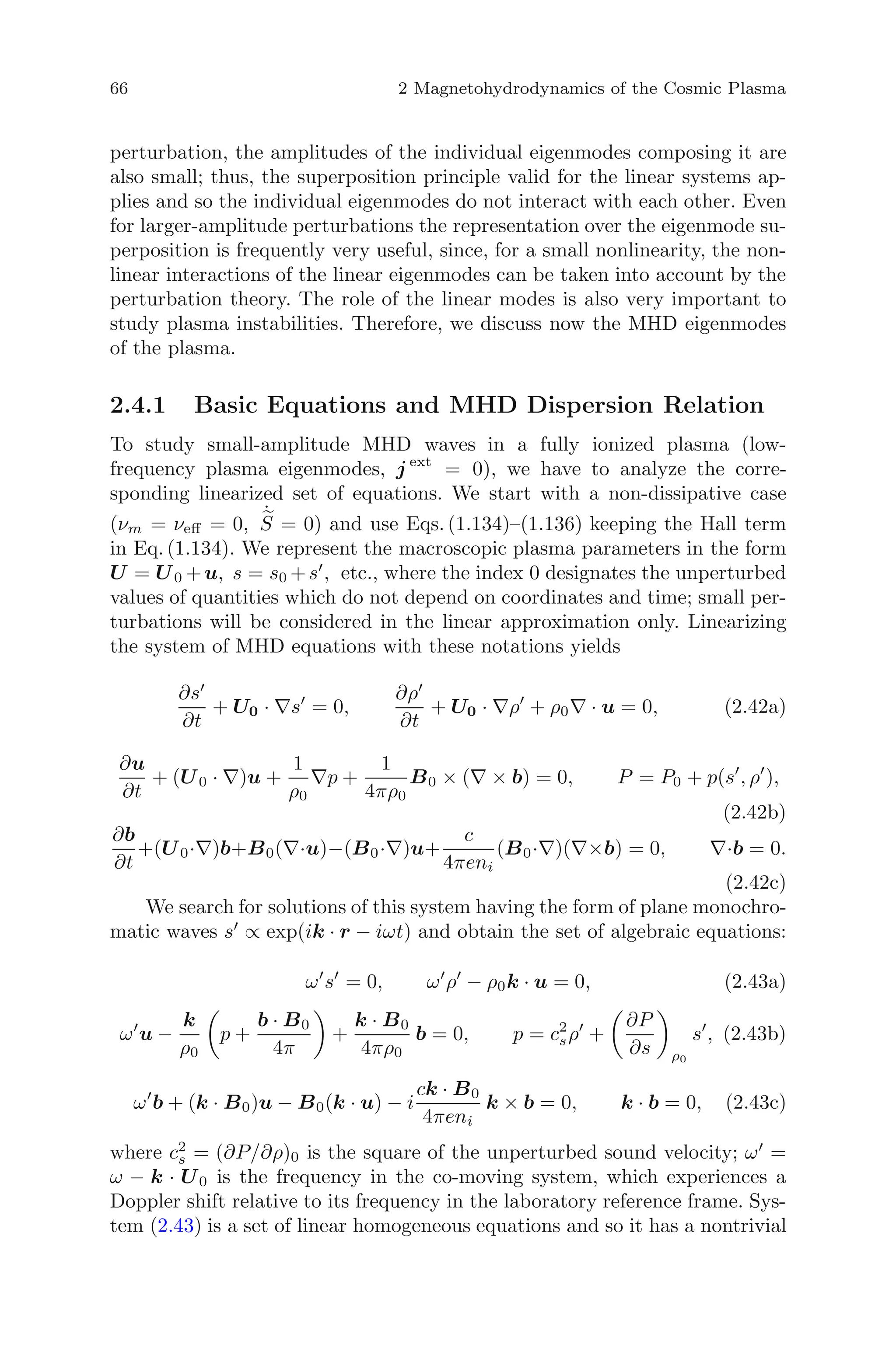
2.4 Linear Modes in MHD
An arbitrary perturbation in a plasma can be expanded over any full system
of orthogonal functions. The most convenient set of such functions, however,
is the set of linear eigenmodes of the medium. Indeed, for a small-amplitude

14. 66 2 Magnetohydrodynamics of the Cosmic Plasma
perturbation, the amplitudes of the individual eigenmodes composing it are
also small; thus, the superposition principle valid for the linear systems ap-
plies and so the individual eigenmodes do not interact with each other. Even
for larger-amplitude perturbations the representation over the eigenmode su-
perposition is frequently very useful, since, for a small nonlinearity, the non-
linear interactions of the linear eigenmodes can be taken into account by the
perturbation theory. The role of the linear modes is also very important to
study plasma instabilities. Therefore, we discuss now the MHD eigenmodes
of the plasma.
2.4.1 Basic Equations and MHD Dispersion Relation
To study small-amplitude MHD waves in a fully ionized plasma (low-
frequency plasma eigenmodes, j ext
= 0), we have to analyze the corre-
sponding linearized set of equations. We start with a non-dissipative case
(νm = νeff = 0,
˙
S = 0) and use Eqs. (1.134)–(1.136) keeping the Hall term
in Eq. (1.134). We represent the macroscopic plasma parameters in the form
U = U0 +u, s = s0 +s , etc., where the index 0 designates the unperturbed
values of quantities which do not depend on coordinates and time; small per-
turbations will be considered in the linear approximation only. Linearizing
the system of MHD equations with these notations yields
∂s
∂t
+ U0 · ∇s = 0,
∂ρ
∂t
+ U0 · ∇ρ + ρ0∇ · u = 0, (2.42a)
∂u
∂t
+ (U0 · ∇)u +
1
ρ0
∇p +
1
4πρ0
B0 × (∇ × b) = 0, P = P0 + p(s , ρ ),
(2.42b)
∂b
∂t
+(U0·∇)b+B0(∇·u)−(B0·∇)u+
c
4πeni
(B0·∇)(∇×b) = 0, ∇·b = 0.
(2.42c)
We search for solutions of this system having the form of plane monochro-
matic waves s ∝ exp(ik · r − iωt) and obtain the set of algebraic equations:
ω s = 0, ω ρ − ρ0k · u = 0, (2.43a)
ω u −
k
ρ0
p +
b · B0
4π
+
k · B0
4πρ0
b = 0, p = c2
sρ +
∂P
∂s ρ0
s , (2.43b)
ω b + (k · B0)u − B0(k · u) − i
ck · B0
4πeni
k × b = 0, k · b = 0, (2.43c)
where c2
s = (∂P/∂ρ)0 is the square of the unperturbed sound velocity; ω =
ω − k · U0 is the frequency in the co-moving system, which experiences a
Doppler shift relative to its frequency in the laboratory reference frame. Sys-
tem (2.43) is a set of linear homogeneous equations and so it has a nontrivial

15. 2.4 Linear Modes in MHD 67
solution only when the determinant of the system is zero. Neglecting the Hall
term, the determinant is derived, e.g., in Somov (2006):
ω 2
[ω 2
− (kvA)2
][ω 4
− k2
(c2
s + v2
A)ω 2
+ k2
c2
s(kvA)2
] = 0,
where vA = B0/
√
4πρ0 is the Alfv´en speed. This equation can have four
nonnegative roots, describing four linear MHD modes, which we consider be-
low in more detail. In what follows, complementary to Somov (2006) analysis,
we derive properties of the small-amplitude waves directly from the full
system (with the Hall term) without explicit use of the determinant.
2.4.2 Dispersion and Polarization of Linear Modes
Hydrodynamics Case: B0 = 0
Let us start from a simpler case, when no magnetic field is present in the
plasma; vA = 0. Then, the terms containing vA drop out from the dispersion
relation, which reduces to
ω 6
(ω 2
− k2
c2
s) = 0.
Evidently, this dispersion equation describes two distinct eigenmodes,
corresponding to two its different solutions: ω = 0 and ω 2
= k2
c2
s.
Entropy and Vortex Perturbations If we suppose in Eq. (2.43) that
B0 = 0 and s = 0, we obtain ω = 0, i.e., ω = k · U0. This means that
entropy perturbations are motionless relative to the plasma and propagate
with the velocity of the medium motion, U0. Also, k · u = 0, k · b = 0, and
p = 0, but the density perturbation ρ = 0 and it is defined by s .
Note that the root ω = 0 is triple degenerate, since it originates from
equation ω 6
= 0. Therefore, two more eigenmodes must be present. Indeed,
for ω = 0, the system (2.43) allows having nonzero values of the components
u⊥ and b⊥ transverse to k. Thus, in the general case k × b = 0 and k × u =
0, so, in addition to the entropy perturbation, there are two more vortex
perturbations traveling with the plasma velocity, namely ∇ × b and ∇ × u.
In the absence of B0, they are independent from each other and from the
perturbation of s . It is interesting that even though no regular magnetic
field is present in this case, the small perturbations of the magnetic field
still can exist in the form of eddies (∇ × b), which is a direct consequence
of the fact that our linearized equations were obtained from more general
MHD equations rather than from standard HD equations; in the latter case
no magnetic perturbation would enter the linearized equations at all.
Sound Waves For s = 0, perturbations oscillate with ω = 0. If, as before,
B0 = 0 then for ω = 0, it follows from Eq. (2.43) that b = 0 and u⊥ = 0,

16. 68 2 Magnetohydrodynamics of the Cosmic Plasma
but the perturbations u and ρ satisfy
ω ρ − ρ0ku = 0, c2
skρ − ρ0ω u = 0, (2.44)
which describes sound waves with the dispersion law
ω 2
= (csk)2
, ω = ±csk + k · U0. (2.45)
MHD Case: B0 = 0
Entropy Perturbations in a Magnetic Field For s = 0 and k ·B0 = 0
we find from Eq. (2.43) that ω = k · U0 and thus
p +
b · B0
4π
k −
k · B0
4π
b = 0. (2.46)
Vector k is orthogonal to b, so Eq. (2.46) is equivalent to two equations:
(k · B0)b = 0, p +
b · B0
4π
= 0. (2.47)
If b = 0, (k · B0) = 0, we have from Eqs. (2.47) and (2.43) u = 0, p = 0.
Perturbations of the density and entropy are connected to each other by the
condition p = 0.
If b = 0, (k · B0) = 0, we obtain from Eq. (2.47) that perturbations of
the full pressure are zero:
p +
b · B0
4π
= 0,
but in the general case ρ = 0 and p = 0. It is easy to check that the vortex
perturbations, ∇ × b and ∇ × u, can exist now independently from s and
from each other. The simplest example of the entropy’s perturbation is the
transfer of heated cloud by medium motion.
Alfv´en Waves Now we consider perturbations in which s = 0 and ρ =
0 but ω = 0. Constancy of mass density is the main generic attribute of
the Alfv´en waves. It follows from Eq. (2.43) that b · B0 = 0; i.e., b ⊥ B0.
Since b ⊥ k as well, the perturbations are polarized, in the sense that b is
perpendicular to the plane (k, B0). The amplitudes u and b satisfy
u = −
k · B0
4πρ0ω
b, k · u = 0, (2.48a)
ω b + (k · B0)u − i
c (k · B0)
4πeni
k × b = 0, k · b = 0. (2.48b)

17. 2.4 Linear Modes in MHD 69
Excluding the velocity u from Eq. (2.48b), we obtain
ω 2
−
(k · B0)2
4πρ0
b − i
c ω (k · B0)
4πeni
k × b = 0 (2.49)
and further
k × b = −i
c ω k2
(k · B0)
4πeni(ω 2 − ω2
A)
b, ω2
A =
(k · B0)2
4πρ0
. (2.50)
From last two equalities we find dispersion equation
ω 2
− ω
ω2
Ak
ωBik
− ω 2
A = 0, (2.51)
where ρ0 ≈ mini and ωBi = eB0/mic is the ion cyclotron frequency.
The solution of Eq. (2.51) is
ω = ωA[ξ ± 1 + ξ2], where ξ =
ωAk
2ωBik
=
(k · vA)k
2ωBik
. (2.52)
Here the parameter ξ = vAk/2ωBi is expressed via the Alfv´en velocity:
vA =
B0
√
4πρ0
. (2.53)
It is small, ξ 1, if k 2ωBi/vA and λ = 2π/k vA/πωBi = λc. Note
that parameter ξ is a result of accounting of the Hall current in the MHD
equations. The scale λc is often small compared with other characteristic
scales in astrophysics, which allows neglecting the corresponding Hall term.
For example, in the “warm” phase of galactic disk λc ≈ 3 × 107
cm is even
smaller than the gyroradius of thermal protons, ≈108
cm, for T ≈ 1 eV, B0 ≈
3 μG; thus for certain plasmas the Hall term can be safely neglected in the
entire range of the MHD applicability (recall that the MHD treatment is only
correct if the wavelength is larger than the proton gyroradius).
Neglecting the small parameter ξ in Eq. (2.52) for k 2ωBi/vA we obtain
simpler dispersion law for the Alfv´en waves:
ω = ±
|k · B0|
√
4πρ0
= ±|k · vg|, (2.54)
where vg = ±vA is the group velocity of the Alfv´en waves. Its phase velocity is
vph = ±
B0| cos θ|k
√
4πρ0k
, (2.55)

18. 70 2 Magnetohydrodynamics of the Cosmic Plasma
where θ is the angle between k and B0. According to Eqs.(2.48a) and (2.54),
the velocity u and the magnetic field b in the Alfv´en wave are connected by
a simple dependence:
u = ∓
b
√
4πρ0
. (2.56)
The minus sign in this formula refers to the same sign for ω and k · vA,
and the plus sign refers to different signs for their values. In Alfv´en waves
the curls ∇ × u and ∇ × b are not independent and both propagate with the
Alfv´en velocity relative to the plasma.
If the medium contains a significant portion of neutral atoms, the Alfv´en
velocity depends on the entire mass density ρ ≈ nimi + nama only for the
wavelengths λ > Λia, where Λia is the mean free path of the ions relative to
collisions with the neutrals. In the case λ < Λia the motion of charged com-
ponent is only weakly coupled with the motion of neutral atoms, so the true
one-fluid description of the medium is not possible. The Alfv´en waves with
λ Λia
may exist in the charged subsystem only, and the Alfv´en velocity will be
determined by the ion mass density alone, ρ ≈ nimi.
Magnetic Sound For s = 0 but ρ = 0 we find from Eq. (2.43) that
ω ρ − ρ0k · u = 0, k · b = 0, (2.57a)
c2
skρ − ρ0ω u +
k(B0 · b)
4π
−
(k · B0)b
4π
= 0, (2.57b)
(k · B0)u − B0(k · u) + ω b = 0. (2.57c)
We again neglect here the Hall current, which is valid at low frequencies.
Excluding the perturbation ρ and multiplying Eqs. (2.57b) and (2.57c) by
e0 = B0/B0, we obtain two equations for the parallel components u and b :
c2
sk2
B0k
4πρ0(ω 2 − c2
sk2)
b − ω u = 0, (2.58a)
ω 2
− c2
sk2
− v2
Ak2
ω 2 − c2
sk2
ω b + B0k u = 0. (2.58b)
Exclusion of u leads to dispersion equation
ω 4
− ω 2
(c2
s + v2
A)k2
+ c2
sv2
Ak4
cos2
θ = 0, (2.59)
where θ is the angle between B0 and k. We find phase velocities v = ω /k of
the fast and slow magnetosonic modes from biquadratic Eq. (2.59):
v2
f,s =
1
2
c2
s + v2
A ± (c2
s + v2
A)2 − 4c2
sv2
A cos2 θ . (2.60)

19. 2.4 Linear Modes in MHD 71
Directions of the vectors b and u can easily be found from the above
equations: b belongs to the plane (k, B0) and perpendicular to the vec-
tor k. The vector u belongs to the same plane, but in general it has both
components parallel and perpendicular to k.
Transverse Propagation For B0=0 and k ⊥ B0, Eq. (2.43) allows both
entropy perturbations (s = 0), considered above, and perturbations of the
MHD parameters independent of the entropy variations. For s = 0, the only
nonzero component of u is that parallel to k, as for normal sound waves. As
follows from Eq. (2.43), the magnitudes ρ and k · u satisfy
ω ρ − ρ0k · u = 0, −
c2
sk2
ρ
ρ0
+ ω −
v2
Ak2
ω
k · u = 0. (2.61)
From this, we determine the dispersion law for the transverse sound:
ω = ±k(c2
s + v2
A)1/2
. (2.62)
The perturbations of the magnetic field are parallel to B0 and proportional
to the density perturbations:
b = B0
ρ
ρ0
. (2.63)
Thus, for transverse propagation, besides the entropy perturbations, it is
possible to have only waves of the usual sound type, in which the velocity of
the plasma is parallel to the direction of propagation. The sound velocity cs
is replaced by (c2
s + v2
A)1/2
, i.e., it is renormalized by the magnetic field.
Longitudinal Propagation For k B0 the system yields two types of
wave in addition to the entropy perturbations: usual sound wave, described
by Eqs. (2.46) and (2.47), on which the magnetic field has no influence, and
MHD waves with u and b perpendicular to both directions k B0. Excluding
velocity
u⊥ =
(kB0)
4πρ0ω
b
from vector equations (2.43), we obtain
(ω 2
− ω2
A)e0 × b + i
(kB0) ck ω
4πeni
b = 0, (2.64)
where ωA is given by Eq. (2.50). Equation (2.64) can be written for the mag-
netic field components (bx, by), b = exbx + ieyby in the form
C1bx−C2by = 0, C2bx−C1by = 0, C1 = ω 2
−ω2
A, C2 =
(kB0) ck ω
4πeni
.
(2.65)

20. 72 2 Magnetohydrodynamics of the Cosmic Plasma
The determinant of this set of linear equations equals zero if C2
2 = C2
1 , i.e.,
by = ±bx. This means that two MHD waves have the circular polarizations
with opposite directions of rotation. The dispersion equation for MHD waves
has the form
(ω 2
− ω2
A)2
= ω 2
ω2
A
ck
ωpi
2
, ω2
pi =
4πe2
ni
mi
. (2.66)
The waves have the frequencies ω ≈ ωA = ±kB0/
√
4πρ0, if contribution of
the Hall current is small: (ck/ωpi)2
1.
The Full Set of Linear Modes With the account of the condition
k · b = 0, the last of equations (2.43) yields two equations when projected on
the axes perpendicular to k. The projection along k gives the identity 0 = 0.
Together with the expression of p in terms of ρ and s , Eqs. (2.43) allow
determining the following seven quantities: s , ρ , u, and two components of
b. In the general case, as we have seen, there are seven different (and linearly
independent) solutions: (1) entropy, (2) two Alfv´en, (3) two fast, and (4) two
slow magnetosonic waves, where the solutions differing in the sign of ω are
considered as different solutions. These solutions comprise the full system
of linear eigenmodes over which any small perturbation can be expanded
(Akhiezer et al. 1975).
Any perturbation of the MHD parameters leads to generation of one
or another MHD mode, and therefore the excitation of modes in cosmic
conditions may be highly diverse depending on the object. Sources of the
MHD waves can include mechanical motions of the plasma, rapid transfor-
mations of energy (outbursts), hydrodynamic instabilities (convection), heat-
ing (solar and stellar winds), rotations, and so on. Secondary MHD modes
are often generated by nonlinear interactions of MHD waves with each other
or with different kinds of nonlinear perturbations (e.g., with shock waves).
MHD modes may also be excited by external currents in the plasma, in-
duced by external sources. Finally, there are purely kinetic mechanisms for
excitation of MHD waves connected with the nonequilibrium distribution
function of a plasma component. For example, strong nonequilibrium rela-
tivistic component (cosmic rays) is capable of generating MHD waves in the
cosmic medium.
2.4.3 Damping of MHD Waves
We consider the most important conditions, when the MHD modes are long
living, i.e., γ ω , where γ is the wave damping rate. To investigate the
MHD wave damping we use Eq. (1.129). The first term on the right-hand side
of Eq. (1.129) is sign alternating and, therefore, goes to zero when averaged
over the volume larger than λ3
= (2π/k)3
. Systematic thermal dissipation Q

21. 2.4 Linear Modes in MHD 73
per unit volume is described by the positive quadratic terms in Eq. (1.129):
Q = T ˙S =
χ(∇T )2
T
+
1
2
ρ0ν
∂uα
∂xβ
+
∂uβ
∂xα
−
2
3
(∇ · u)δαβ
2
+
νm
4π
(∇ × b)
2
+
νeff
4π
(∇ × b)
2
⊥ . (2.67)
The thermal dissipation includes three distinct dissipative processes: heat
conductivity, viscosity, and Joule heating.
The damping rate γ, which describes a weak damping of the plane
monochromatic waves in stationary plasma, can be calculated from
γ = Q/2w, (2.68)
where w is the density of the wave energy; the bar over it indicates the
mean amplitude over the period. The magnitude of γ describes exponential
damping of MHD parameters when all the wave sources are off, e.g., u =
u0 exp(−γt) or w ∝ exp(−2γt) for quadratic measures like the energy density.
Another kind of damping measures is the absorption coefficient per unit
path length of the wave propagation:
α = Q/q, (2.69)
where q is the mean absolute value of the wave energy flux. This value
characterizes exponential decrease of the wave amplitude in space, u =
u0 exp(−αz), as the wave propagates from the source. Here, we select the
z-axes along the direction of the energy flux q. The general expressions for
energy density and energy flux density are well known (Landau and Lifshitz
1966; see also Sect. 1.3.3):
w = ρ
1
2
u2
+ +
B2
8π
, (2.70a)
q = ρu
1
2
u2
+ +
P
ρ
+
1
4π
B × (u × B), (2.70b)
where is the internal energy per unit mass and +P/ρ is the enthalpy. This
energy flux does not include the dissipative terms.
It is now easy to apply these general formulae to derive the damping
rates of the MHD waves; we list the final results only for the sake of brevity.
Sound Waves: B0 = 0
γs =
1
2
k2 4
3
ν +
χ
ρ
(c−1
V − c−1
P ) , (2.71)
where cV and cP are the specific heats at constant volume and pressure,
respectively. The absorption coefficient per unit path length is αs = γs/cs,
where cs is the group velocity of the sound wave.

22. 74 2 Magnetohydrodynamics of the Cosmic Plasma
Alfv´en Waves
γA =
1
2
(νk2
+ νmk2
⊥ + νeffk2
). (2.72)
If neutral atoms are present, the damping is primarily accounted for by the
high effective collisional viscosity. This takes place for k2
/k2
⊥ νm/νeff.
In the absence of the neutral component (νm = νeff) we obtain standard
expression γA = (ν + νm)k2
/2.
Magnetosonic Waves For simplicity we suppose c2
s v2
A, omit the kine-
matic viscosity and the heat conductivity, while take into account the mag-
netic diffusivity, which yields
γf =
1
2
νeffk2
, γslow =
c2
s
2v2
A
νeffk2
⊥. (2.73)
If k⊥ → 0, expression (2.73) gives γslow → 0 in this approximations. In fact,
the slow magnetosonic wave converts here to the usual sound wave and so
damping rate Eq. (2.71) applies.
2.5 Solar and Stellar Winds
Plasma motions allowing the MHD description are highly typical for the
astrophysics context. Many objects (typically, those with fast rotation) form
accretion disks and produce collimated flows of the plasma—astrophysical
jets; others produce more isotropic winds. We emphasize that both these
kinds of the plasma outflows are very common. The jets are observed or
implied in galactic microquasars, in active galactic nuclei, quasars, blazars,
and gamma-ray burst sources; see Sect. 12.4. In many cases the plasma moves
with relativistic or even ultrarelativistic speed in these jets.
More isotropic winds are typical for galaxies and normal stars (e.g.,
Fig. 1.3), although neutron stars produce ultrarelativistic “pulsar winds” in
some cases, resulting in a phenomenon of pulsar wind nebulae (e.g., Figs. 1.6
and 1.7 and Sect. 12.3). As a simpler example, we consider here nonrelativistic
winds of the normal stars.
The idea of stellar/solar wind had been around well before the space era;
however, it was not clear if the corpuscular flows from stars are sporadic or
persistent. Direct measurement of the persistent corpuscular flow from the
Sun was performed in Greenhouse’s experiment on board Sputnik “Luna-2”
in 1959 and then confirmed by satellite Mariner-2 measurements. Soon af-
ter this fundamental discovery, the stellar winds were detected (indirectly)
from stars of spectral types O and B during the 1960s of the twentieth cen-
tury. It was established that many (most of the) hot massive (M 10M )
high-luminosity stars produce their winds with a very large mass loss rate
(Lozinskaya 1992). For example, for the Wolf–Rayet (WR) and Of stars the

23. 2.5 Solar and Stellar Winds 75
mass loss rate is about ˙M ≈ (10−5
–10−4
) M /year; thus, the star can lose
a considerable fraction of its mass over time of the order of 106
years that
is very modest time compared with other astronomic timescales. For exam-
ple, the Earth are known to exist about 4.5 × 109
years, while the Sun has
been shining even longer. The stellar wind speeds were found to range within
u ≈ (1–4)×103
km/s. This implies a major deposition of the wind energy into
the interstellar medium: with the above values one can easily estimate that
the stellar wind energy deposition over the star lifetime, ∼106
years, is around
(0.1–10)×1051
erg, which is comparable with the energy released during the
supernova explosion occurring at the end of the massive star evolution.
Thus, the stellar wind is not a minor effect; rather it can have numerous
dynamical and evolutionary implications. For example, the rapid mass loss,
(10−5
–10−6
)M /year, affects the star evolution itself including the end of
its evolution—supernova explosion, and the supernova remnant expansion—
which occurs in a “preprocessed” circumstellar cavity filled by the stellar wind
rather than in an average interstellar medium. That strong stellar winds affect
the interstellar medium by the deposition of energy and chemical elements
and disturbing its dynamics parameters, including the ISM magnetic field.
Given that the massive stars are not randomly distributed in the Galaxy, but
correlated within so-called OB associations, the stellar winds from different
stars can interact with each other and merge into a powerful velocity field
additionally enhanced by supernova explosions within the association. These
interacting winds form a bubble (also called “superbubble”) with a linear
scale up to a few hundred pc, which is bounded by a cooler supershell ex-
panding as a single object due to cumulative pressure produced by the winds
and explosions. We will be returning to these phenomena below in the book.
Although hundreds of stars with high luminosity L within (5 × 102
–5 ×
107
)L were observed to produce the winds with the mass rate within ˙M ≈
10−9
M /year and ˙M ≈ 10−4
M /year, the mass losses in the form of the
wind are also typical for stars with much weaker luminosity. For example,
observations favor winds from much less luminous stars, e.g., cool massive red
giants ( ˙M ≈ 10−6
M /year, u ≈ 10 km/s), from nuclei of planetary nebulae
with the speed (2–3)×103
km/s (which is 3–4 times larger than the gravitation
runaway velocity) and the mass loss rate ˙M ≈ (4 × 10−9
–7 × 10−7
)M /year,
and, finally, from the closest to the Earth star, the Sun.
2.5.1 Basic Observational Data About
the Solar Wind
The solar wind is one of the main constituents which, along with eruptive
phenomena and electromagnetic radiation from the Sun and planets, deter-
mines physical conditions in the circumsolar space (Fig. 1.3). The solar wind
is a more or less stationary and isotropic plasma flow, which is launched in the
upper corona of the Sun and transfers magnetic fields of solar origin. The first

24. 76 2 Magnetohydrodynamics of the Cosmic Plasma
indications of some corpuscular flow outward the Sun in interplanetary space
were obtained in the nineteenth century (e.g., see Brandt 1970 for a review).
The persistent character of the solar wind was experimentally established by
Biermann (1951, 1952) via investigation of the behavior of comet tails. This
result was further confirmed indirectly by observations of modulation of the
galactic cosmic rays and by data on geomagnetic activity and auroras.
Direct measurements of the interplanetary plasma parameters became
possible in the space era by Earth-orbiting satellites and also by interplane-
tary spacecraft missions. They provide quasi-continuous measurements of the
interplanetary plasma physical parameters in various locations of the space.
Remarkably, the parameters of the solar wind, the particle number density,
abundances, velocity, and temperature experience significant temporal and
spatial variations. Nowadays, the running combination of the involved IPM
parameters and their drivers are collectively called the “space weather”(Gary
and Keller 2004).
The measurements at the Earth orbit give the solar wind velocity (mass
velocity) u between ≈ 300 and ≈ 700 km/s (the mean value is ≈ 400 km/s; the
highest values of ≈ 2,000 km/s are measured in association with sequences
of largest solar flares, e.g., in November 2003); the ion number density ≈
5 cm−3
; the flux density of positive ions 2×108
cm−2
s−1
and the temperature
Tp ≈ 3 × 104
–6 × 105
K (the mean value is 1.5 × 105
K) for protons and
Te ≈ 1.5 × 105
for electrons. The number density of He++
ions (the α-
particles) is usually around 4–5 % of the proton number density. The number
of neutral atoms is insignificant. The magnetic field is measured to be highly
variable and typically to belong the range (1–10)×10−5
G with the mean value
of B ≈ 5 × 10−5
G. Solar wind is a supersonic flow, whose Mach numbers
M = u/vT i and MA = u/vA have values 8–10.
The numbers allow estimating typical values of the solar wind kinetic
energy density nimiu2
/2 ≈ 10−9
erg cm−3
and the magnetic energy density
B2
/8π ≈ 10−10
erg cm−3
near the Earth orbit, so the kinetic energy of the
hydrodynamic flow exceeds the magnetic energy by a factor of ten. This al-
lows neglecting the electromagnetic forces and considering the solar wind as
a purely hydrodynamic flow to the first approximation. But before applying
the HD we have to check if condition (2.9) Λii r is fulfilled, where r is helio-
centric distance and Λii is the ion mean free path. We have Λii = 1/niσii and
use the Coulomb cross section σii ≈ π(e2
/miv2
T i)2
ln ΛC ≈ π(e2
/Ti)2
ln ΛC
obtained for the thermal plasma (see Sect. 1.3.7). It is then convenient to
express the mean free path Λii in astronomical units (1 AU ≈ 1.49×1013
cm):
Λii ≈ 0.7 × 10−9
T 2
i /ni, (2.74)
where the temperature and the number density are in Kelvin and cm−3
,
respectively.
Adopting the coronal values ni = 2 × 108
cm−3
and Ti = 2 × 106
K for
the height at which the solar wind is launched, we obtain Λii ≈ 2 × 108
cm

25. 2.5 Solar and Stellar Winds 77
R ≈ 7 × 1010
cm; thus, the hydrodynamic description is applicable here.
However, at the Earth orbit, we have Ti ≈ 105
K and ni ≈ 5 cm−3
. Formula
(2.74) gives Λii ≈ 1 AU in this case, i.e., Λii ≈ r, so the space plasma is
collisionless and the hydrodynamic approach seems to fail. Nevertheless, as
we have discussed in Sect. 1.3.8, the anomalous processes can strongly reduce
the particle mean free path in the collisionless plasma compared with that
determined by the Coulomb scattering only. Fluctuations of interplanetary
magnetic field and plasma waves developed due to different plasma instabil-
ities make the particle trajectories tangled and the velocities more isotropic,
and so reduce their mean free paths, which ensures broader applicability of
the HD/MHD approach than it could be anticipated. Complementary, the
effective mean free path of solar wind protons was measured from experi-
mental data about its distribution function (see, e.g., the first data reported
by Brandt et al. 1973; Marsch et al. 1982a,b). The anomalous mean free path
varies depending on the IPM state and was found to be well below 0.1 AU
in many cases. This remarkable finding justifies approximate applicability of
the standard HD equations to describe the solar wind at 1 AU and farther
away from the Sun.
It should be emphasized, however, that for the number densities and
temperatures typical for the interplanetary plasma, the mean free path of
particles with respect to Coulomb collisions is rather large and often exceeds
1 AU. Thus, the particle distributions are not necessarily isotropic, and par-
ticle distribution functions are not necessarily Maxwellian (see Sect. 1.3.8).
In agreement with this expectation, the measured steady-state distribution
function of the solar wind particles is typically well described by a kappa
distribution, rather than a Maxwellian. The thermal energies of electrons
and ions (i.e., the electron and ion effective temperatures) are often differ-
ent. This means that the solar wind is seldom (never) in a state of a true
thermodynamic equilibrium.
We note that the Sun loses an extremely small part of its mass in the
form of the solar wind. The discussed parameters of the solar wind allow
estimating the entire mass flow from the Sun: JM = 4πr2
0umini ≈ 1019
g/year
≈ 10−14
M /year, where r0 = 1 AU, M ≈ 2 × 1033
g is the solar mass.
During the Sun lifetime (<1010
years) the solar wind has taken out total of
only 10−4
M if we adopt that the flow parameters are more or less constant
over this time.
2.5.2 Parker’s Model of the Solar Corona
Expansion
Let us apply, following Parker (1963), the HD equations to understand the
phenomenon of the solar wind. We start with analysis of the hydrostatic
(∂/∂t = 0 and u = 0) equilibrium of a spherically symmetric fully
ionized hydrogen atmosphere to which the equation of state, Eq. (2.23),

26. 78 2 Magnetohydrodynamics of the Cosmic Plasma
P(r) = 2ni(r)T (r) of a tenuous gas applies. Neglecting electromagnetic
forces, Eq. (2.2) requires that the pressure gradient is balanced by the
gravitation force:
d
dr
2niT +
GM mini
r2
= 0, (2.75)
where G ≈ 6.67 × 10−8
cm3
g−1
s2
=6.67 × 10−11
m3
kg−1
s2
is the gravitational
constant. Integration of this equation yields
ni(r)T (r) = ni(r0)T (r0) exp −
GM mi
2
r
r0
ds
s2T (s)
. (2.76)
Remarkable conclusions about the hydrostatic equilibrium can be derived
from analysis of the rhs of the equation. Indeed, if the temperature T (r) de-
creases with r faster than r−1
then the exponent index decreases infinitely at
r → ∞ and, thus, ni(r)T (r) → 0 at the infinity. Stated another way, this tells
us that the stellar atmosphere has a finite size and a hydrostatic equilibrium
is achievable.2
The only way of the atmosphere dissipation here is gravitation
runaway of higher-energy particles from a “tail” of the steady-state distribu-
tion, which is beyond the HD applicability region.
However, if the temperature decreases slower than r−1
then the exponent
index in Eq. (2.76) has a finite value at arbitrarily large r, which implies a
finite pressure at the infinity. Since a finite gas amount (stellar atmosphere)
cannot be distributed over an infinite volume with a finite density, we arrive
at a conclusion that no hydrostatic equilibrium is possible in this case; thus,
a HD expansion with some u(r) = 0 must appear.
Let us consider this expansion assuming the motion to be stationary
(∂/∂t = 0 as before). We use the equation of mass conservation
ni(r)u(r)r2
= ni(r0)u(r0)r2
0, (2.77)
where r0 is the stellar radius at the base of corona, and the equation of motion
miniu
du
dr
+
d
dr
2niT +
GM mini
r2
= 0. (2.78)
Full solution of the problem requires also an energy transfer equation. How-
ever, the fundamental science question of the mechanisms of the solar wind
heating (and, more generally, of the corona heating) is highly sophisticated
and has not yet been fully understood, which will be discussed in greater de-
tail later. Now, to make a qualitative progress, we adopt a simple power law
for the temperature dependence on r without assuming a specific mechanism
of the corona heating.
2
It must be noted that such hydrostatic equilibrium is not necessarily stable: for
example, it can be convectively unstable if the temperature gradient is large; see
Chap. 6.

27. 2.5 Solar and Stellar Winds 79
It is convenient to introduce two characteristic proton velocities, the ther-
mal speed (which is also the “isothermal” speed of sound)
vT (r) = [2T (r)/mi]1/2
(2.79)
and the runaway velocity from r0
ve = (GM /r0)1/2
= const. (2.80)
With this notations Eq. (2.78) receives the form
u
du
dr
1 −
v2
T
u2
= R(r), (2.81)
where
R(r) = −r2 d
dr
v2
T
r2
−
v2
er0
r2
. (2.82)
We consider the case when the atmosphere is strongly coupled with the
star v2
e v2
T (r0) u2
(r0) at the level r = r0, while the temperature T
monotonously decreases with r slower than r−1
, i.e., T (r) = T0(r/r0)ε−1
,
0 < ε < 1, T (∞) → 0. For r → r0 we have R(r) < 0 because v2
e v2
T .
Nevertheless, the first term in the rhs of Eq. (2.82) is positive and decreases
slower than r−2
. Therefore, a “critical layer” r = rc exists, where R(rc) = 0,
with R(r) > 0 at r > rc and R(r) < 0 at r < rc. Since at the corona base,
r = r0, the expansion is weak, u2
v2
T , then both values entering Eq. (2.81),
1 − v2
T /u2
and R(r), are negative, so du/dr > 0 is positive, i.e., the gas is
being accelerated by the pressure gradient.
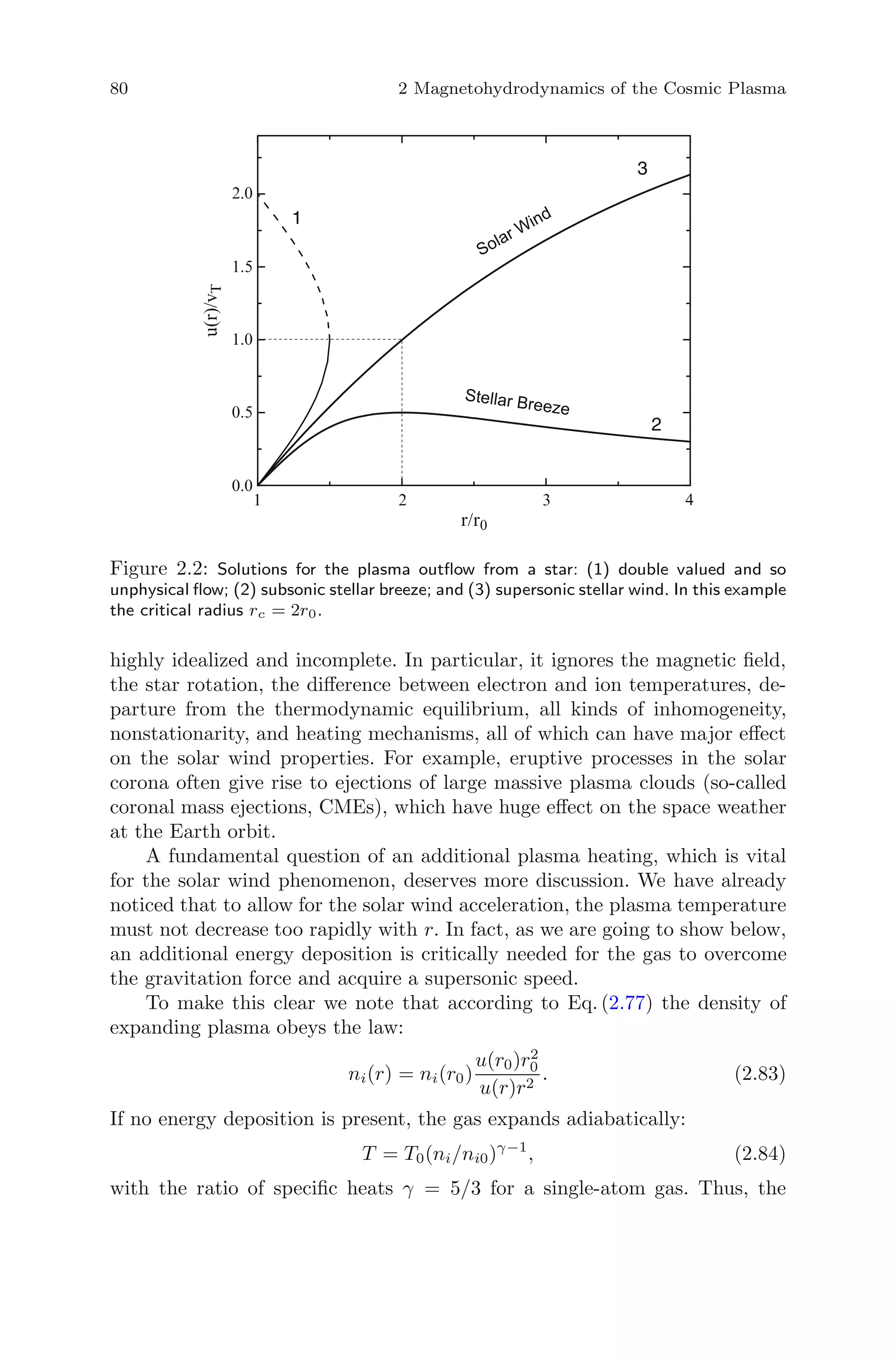
Consider what can happen to the flow farther away from the star. If,
(1) during the gas acceleration, the flow velocity u reaches the value of vT
somewhere at r < rc then du/dr → ∞ at vT = u according to Eq. (2.81),
while the flow velocity is directed toward the star at larger r (see curve 1 in
Fig. 2.2). Such solutions seem to be inconsistent with the adopted stationarity
of the flow and so require account of the time derivative in Eq. (2.2). If (2) the
equality vT = u is not achieved at r < rc, then the derivative du/dr becomes
negative at r > rc, and the gas motion remains subsonic at the entire space
decaying gradually at large distance from the star. Such solutions (see curve
2 in Fig. 2.2) are called the stellar breeze to distinguish from supersonic solar
wind. Finally, (3) if the expansion velocity u reaches the thermal velocity vT at
the very same layer rc, where R(rc) = 0 (curve 3 in Fig. 2.2), then the stellar
wind becomes supersonic at r > rc, where it keeps accelerating. This solution
does correspond (qualitatively) to the solar wind actually observed in the
IPM. For any given temperature profile, one can plot dependences of u and
other relevant parameters on r numerically.
We must emphasize, however, that even though the model considered
uncovers the fundamentals behind the solar wind phenomenon, it remains

28. 80 2 Magnetohydrodynamics of the Cosmic Plasma
1
0.0
0.5
1.0
1.5
2.0
2 3
r/r0
u(r)/vT
4
1
2
3
Figure 2.2: Solutions for the plasma outflow from a star: (1) double valued and so
unphysical flow; (2) subsonic stellar breeze; and (3) supersonic stellar wind. In this example
the critical radius rc = 2r0.
highly idealized and incomplete. In particular, it ignores the magnetic field,
the star rotation, the difference between electron and ion temperatures, de-
parture from the thermodynamic equilibrium, all kinds of inhomogeneity,
nonstationarity, and heating mechanisms, all of which can have major effect
on the solar wind properties. For example, eruptive processes in the solar
corona often give rise to ejections of large massive plasma clouds (so-called
coronal mass ejections, CMEs), which have huge effect on the space weather
at the Earth orbit.
A fundamental question of an additional plasma heating, which is vital
for the solar wind phenomenon, deserves more discussion. We have already
noticed that to allow for the solar wind acceleration, the plasma temperature
must not decrease too rapidly with r. In fact, as we are going to show below,
an additional energy deposition is critically needed for the gas to overcome
the gravitation force and acquire a supersonic speed.
To make this clear we note that according to Eq. (2.77) the density of
expanding plasma obeys the law:
ni(r) = ni(r0)
u(r0)r2
0
u(r)r2
. (2.83)
If no energy deposition is present, the gas expands adiabatically:
T = T0(ni/ni0)γ−1
, (2.84)
with the ratio of specific heats γ = 5/3 for a single-atom gas. Thus, the

29. 2.5 Solar and Stellar Winds 81
temperature decreases as
T ∼ u−(γ−1)
r−2(γ−1)
, (2.85)
i.e., ∝ r−4/3
for a constant expansion velocity and even faster for an acceler-
ated expansion, which is in all the cases faster than a limiting temperature
profile ∝ r−1
obtained from Eq. (2.76).
Let us estimate the required heat deposition based on the energy bal-
ance consideration (Parker 1979). The gravitation energy density per unit
volume is
Φ(r) = −
GM mini
r
. (2.86)
The energy, which is spent for the gas to overcome the gravitation field and
to accelerate the gas, is the enthalpy, which accounts the work of the pressure
force:
w = + P =
2γ
γ − 1
niT. (2.87)
Here = niT/(γ − 1) is the internal energy density. The ratio
w
|Φ(r0)|
=
5T r0
GM mi
≈ 0.43 (2.88)
is less than one for r = r0 ≈ 0.7 × 1011
cm and T ≈ 2 × 106
K and so is
insufficient to produce the wind. Therefore, to overcome the gravitation and
to accelerate then gas up to 400 km/s an additional energy Q must indeed be
deposited. In place of explicit account of the energy sources, we describe this
energy deposition by using the polytropic equation instead the adiabatic one:
T = T0(ni/n0i)α−1
, (2.89)
where α is the polytropic index. For α < γ comparison of Eq. (2.89) with
adiabatic equation (2.84) reveals that for the same gas expansion ni/n0i,
the temperature is larger for polytropic process than for the adiabatic pro-
cess. Therefore, this does account for an additional heat deposition into the
gas, with the heat efficiency defined by the polytropic index; apparently, no
information on the physical mechanisms of the plasma heating is available
in Eq. (2.89) within this treatment.
We can now introduce an effective enthalpy weff accounting for the
additional heat deposition in the form of Eq. (2.87) with the polytropic index
α in place of the adiabatic index: γ
weff =
2α
α − 1
niT. (2.90)

30. 82 2 Magnetohydrodynamics of the Cosmic Plasma
The required polytropic index then can easily be estimated from the energy
conservation per particle at the corona base and far away from the Sun in a
region of the supersonic wind:
2α
α − 1
T0 −
GM mini
r0
=
miu2
(r)
2
. (2.91)
Here we neglected the expansion velocity at the corona base and neglected
thermal energy and gravitation potential far away from the Sun. Substitution
of the mean solar wind speed u(r) = 400 km/s and typical coronal parameters
yields α ≈ 1.14; Parker (1979) proposed 1.0 < α < 1.3 as the most plausible
range for the polytropic indices. Equation (2.91) also tells us that for low
coronal temperature
T0 <
(α − 1)GmiM
2αr0
, (2.92)
the expansion is impossible and the corona remains static.
Let us touch upon possible mechanisms of the additional heat deposition
into the expanding plasma. Generally, there are absorption of the solar ra-
diation flux, standard heat conductivity, losses of nonthermal particle pop-
ulation, and dissipation of various plasma/MHD waves, which are efficiently
generated in the convective zone of the Sun and then transferred outward to
the corona. First three mechanisms are easy to take into account; it turns that
all they are insufficient to provide the required plasma heating. We, therefore,
forced to conclude that the primary source of the heat is the wave dissipa-
tion. However, it is extremely difficult to quantitatively check this conclusion
because the theory of wave generation, propagation, and damping is very
complicated and in addition depends on poorly known details of the solar at-
mosphere structure and relevant physical conditions. We will consider some
of the related processes and phenomena below in this book; however, the cur-
rent state of the science is yet unable to fully describe the phenomenon of the
solar wind and in particular—reliably identify the sources and mechanisms
of the additional corona heating.
The discussed simplest model of the uniform corona expansion suggests
that the solar wind overcomes the sound speed and becomes supersonic at
around rc ≈ 10r . Accordingly, at the Earth orbit, the plasma flow is highly
supersonic and superalfvenic. We note that a very interesting physics takes
place at those regions where such a supersonic flow interacts with an obstacle.
A practically important and actively studied example of this is the interaction
of the solar wind with the Earth’s magnetosphere (Fig. 1.3), which results in
a variety of observable manifestations including the polar lights (Fig. 1.4).
Then, as the wind propagates farther away from the Sun, the ISM
surrounding the solar system starts to affect and modify the solar wind
(see, e.g., Hundhausen 1972; Baranov and Krasnobaev 1977). Indeed, if the
interstellar medium pressure were absent, the solar wind speed would remain

31. 2.5 Solar and Stellar Winds 83
approximately constant, of the order of 400 km s−1
; its number density would
fall with distance as r−2
, and the temperature would also decrease as de-
scribed. Hence, the solar wind would become more and more supersonic.
However, in the real situation, the solar wind is slowed down by the inter-
stellar medium and, therefore, the supersonic regime should give a way to a
subsonic one at some distance from the Sun, which is accompanied by the
appearance of a termination shock.
A rough estimate of the shock position rsh may be obtained from
the requirement of balance between the solar wind dynamic pressure and
interstellar medium pressure:
nimiu2
≈ (na + 2ne)T +
B2
8π
+ PCR, (2.93)
where PCR is the cosmic ray (relativistic particles) pressure, na is the number
density of neutral atoms in interstellar medium, ne is the electron number
density in interstellar medium, and T is its temperature. Substituting ni =
niEr−2
, where niE ≈ 5 cm−3
and rT sh is the distance in AU, and other
parameters adopted above, we obtain rT sh ≈ 100 AU.
A number of space missions have been launched toward the anticipated
bounds of the solar system years ago to determine where those bounds are
and what are the physical conditions there. The first reliable detection of the
termination shock occurred on December 14, 2004, by a spacecraft Voyager 1
at the distance 94 AU from the Sun. It took around 30 years for the spacecraft,
launched on 1977, to path through the solar system. Later, Voyager 2 having
a different trajectory detected the termination shock at the distance 84 AU
on August 30, 2007. In fact, Voyager 2 detected the termination shock a few
times: this is because the position of the termination shock is changing in
time in response to short-term variations of the solar activity. It is supposed
that the shock position also experiences systematic changes back and forth
following the 11 years cycle of the solar activity. According to the measure-
ments made by Voyagers 1 and 2, the solar wind velocity near the heliospheric
shock wave was approximately 380 km/s, and the ratio u1/u2 = ρ2/ρ1 ≈ 3
at the front.
2.5.3 Magnetic Field in a Cavity Filled
by a Stellar Wind
Consider now another important constituent of the solar wind, the mean mag-
netic field. Specifically, let us apply dissipation-free induction equations (2.33)
to calculate the magnetic field structure in a volume filled by solar or stellar
wind within a simple model. Here, we adopt that the plasma is launched
isotropically from a spherical surface of the radius a, rotating around a central
axes with constant angular velocity Ω. The stellar wind speed u is constant
and has radial direction. At the spherical surface there is a magnetic field,

32. 84 2 Magnetohydrodynamics of the Cosmic Plasma
which is described by the function B(a, ϑ, α) = B0(ϑ, α) in the reference
frame rotating together with the star, where α is the azimuth angle in the
plane transverse to the rotation axes. The energy density of the plasma mo-
tion exceeds significantly the energy density of the magnetic field; thus, we can
neglect the magnetic field effect on the plasma motion. Using the freezing-in
condition we find here the magnetic field distribution (dependence of the mag-
netic field on the coordinates and time) in the region r > a in the laboratory
(rest frame) system.3
To solve this problem we first project vector equation (2.38) to the axes
r and substitute u = ur/r, u = const, which yields the equation for Br:
∂Br
∂t
= −
2u
r
Br − u
∂Br
∂r
. (2.94)
Solution of this equation is an arbitrary function of independent variables
r − ut, ϑ, and α divided by r2
:
Br(r, ϑ, α, t) =
1
r2
F(r − ut, ϑ, α). (2.95)
The boundary condition has evidently the form
Br r=a
= B0r(ϑ, α + Ωt) =
1
a2
F(a − ut, ϑ, α), (2.96)
where the argument α + Ωt in B0r originates from the transition from the
rotating frame to the laboratory rest frame; therefore
F(a − ut, ϑ, α) = a2
B0r(ϑ, α + Ωt)
and solution (2.95) reads
Br(r, ϑ, α, t) =
a
r
2
B0r ϑ, α −
(r − a)Ω
u
+ Ωt . (2.97)
In a similar way, we find two remaining components of the magnetic field:
Bϑ =
a
r
B0ϑ ϑ, α −
(r − a)Ω
u
+ Ωt , (2.98a)
Bα =
a
r
B0α ϑ, α −
(r − a)Ω
u
+ Ωt . (2.98b)
3
The model considered here was proposed by Parker (1959) to describe the in-
terplanetary magnetic field produced by the solar plasma flows composing the solar
wind.

33. 2.5 Solar and Stellar Winds 85
Figure 2.3: Two oppositely directed magnetic field lines illustrating the Parker model
of the IPM magnetic field at the scale of the Earth (left) and Jupiter (right) orbits. The
planet orbits are shown by dashed color circles (the orbit eccentricities are neglected) for
Mercury (grey), Venus (violet), Earth (bold blue; the planet itself is shown by blue circle;
not in scale), Mars (red), and Jupiter (brown).
Using Maxwell equation ∇ · B = 0 and Eq. (2.97) gives rise to the following
useful relationship between components of the vector B0:
−
aΩ
u
∂B0r
∂α
sin ϑ +
∂
∂ϑ
(B0ϑ sin ϑ) +
∂B0α
∂α
= 0.
For example, if B0ϑ = 0 then Bϑ = 0 during the entire field evolution, and
B0α =
aΩ
u
B0r sin ϑ + f(ϑ).
If we further adopt f(ϑ) = 0, we then obtain
Bα(r, ϑ, α, t) =
a2
Ω
ur
B0r ϑ, α −
(r − a)Ω
u
+ Ωt sin ϑ. (2.99)
Equations (2.97) and (2.99) show that the azimuth component of the
magnetic field decreases with r much slower, as ∝ r−1
, than the radial
component does, as ∝ r−2
. Thus, even if the radial component of the mag-
netic field dominates at the star surface, the azimuth component dominates
farther away from the star, which gives rise to the spiral shape of the mean
interplanetary magnetic field.
Parker applied this model to describe the interplanetary magnetic field
of the solar wind (Fig. 2.3). The original Parker’s model adopts Bϑ = 0,
while Br and Bα are described by Eqs. (2.97) and (2.99). Measurements of
the interplanetary magnetic field indicate the presence of a slowly varying

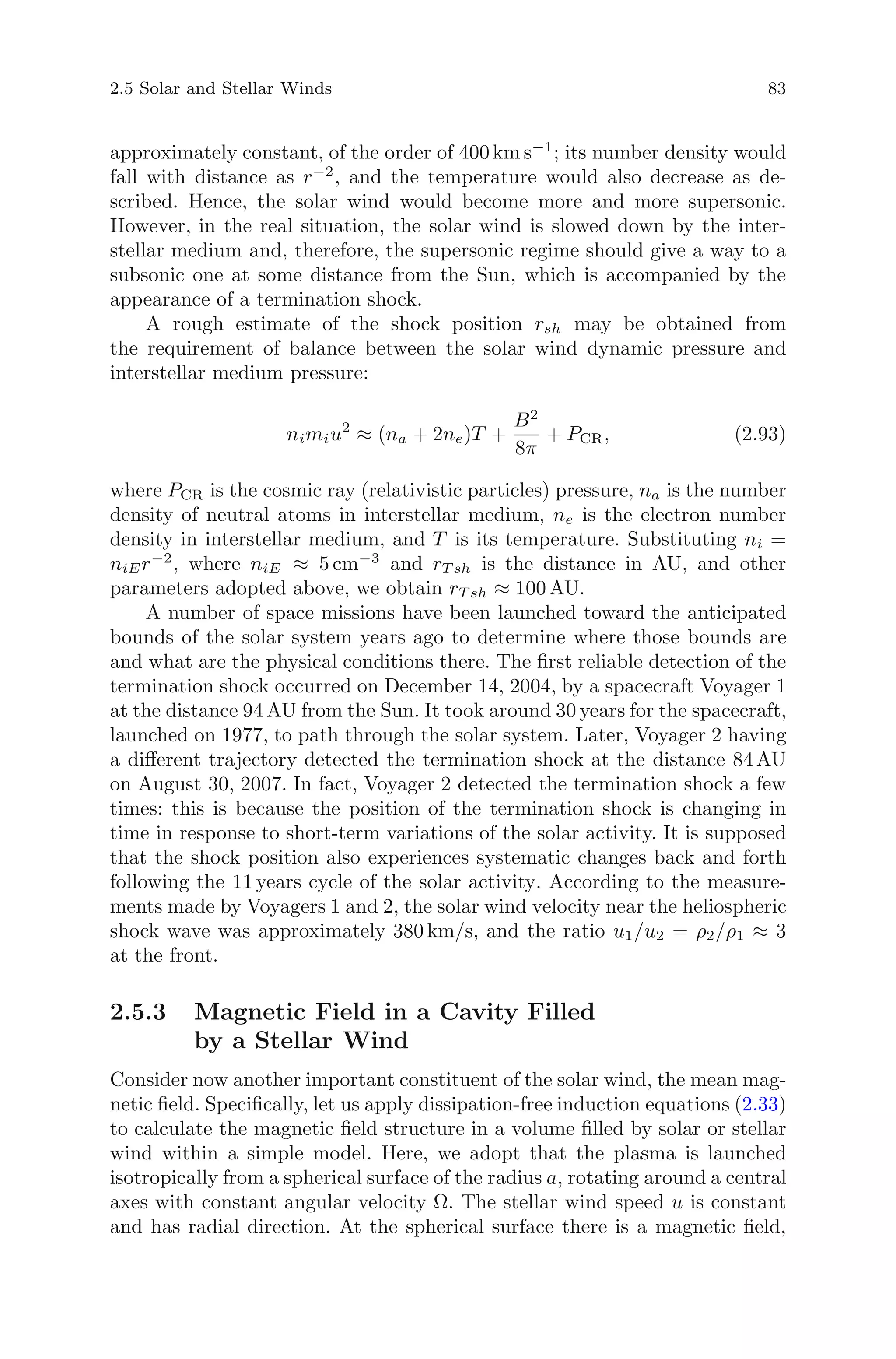
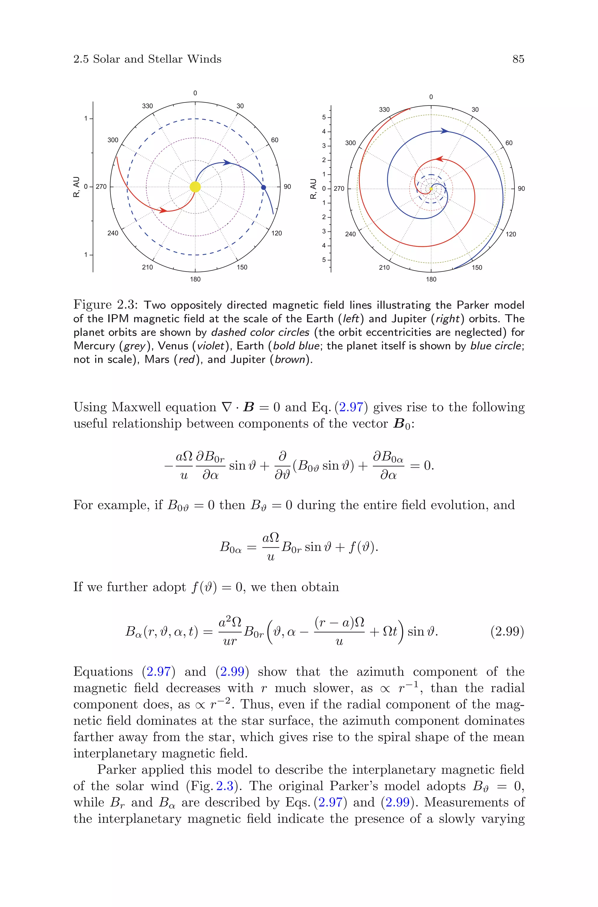
34. 86 2 Magnetohydrodynamics of the Cosmic Plasma
component, which indeed has an approximately spiral structure and inter-
sects the Earth orbit at an angle of 45◦
. The average magnetic field near the
Earth orbit is close to 5 × 10−5
G, though the measured values are scattered
very strongly. At low heliographic latitudes the spiral field consists of several
sectors with mutually opposite magnetic field directions. The radial compo-
nent varies with distance as r−2
, in good agreement with the Parker model.
However, the agreement is much poorer for the azimuthal component, which
displays the dependences from Bα ∼ r−1.23
to ∼ r−1.1
between 1 and 5 AU.
The component Bϑ < 10−5
G was also observed near the Earth orbit.
The magnetic field structure unlike the solar wind itself is not spheri-
cally symmetric. Given that the magnetic energy density is one–two orders
of magnitude smaller than the kinetic energy of the solar wind, thus, a rela-
tively weak deviation of the solar wind from the spherically symmetric flow
can have major effect on the magnetic field structure. Even though obser-
vations do often reveal significant departure of the measured magnetic field
from the Parker’s one, the overall agreement is, nevertheless, remarkably good
especially if one takes into account the number of the simplifications adopted.
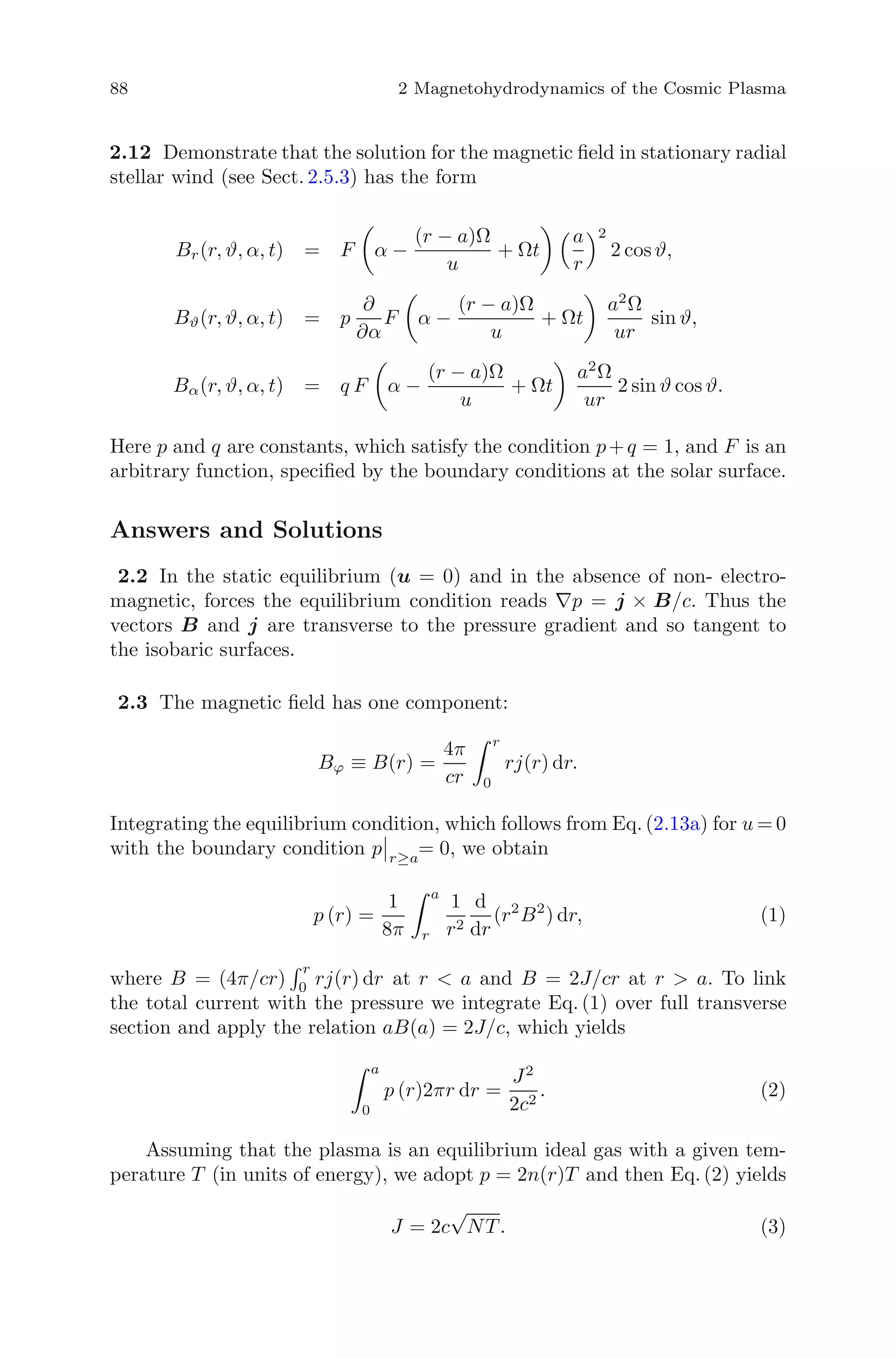
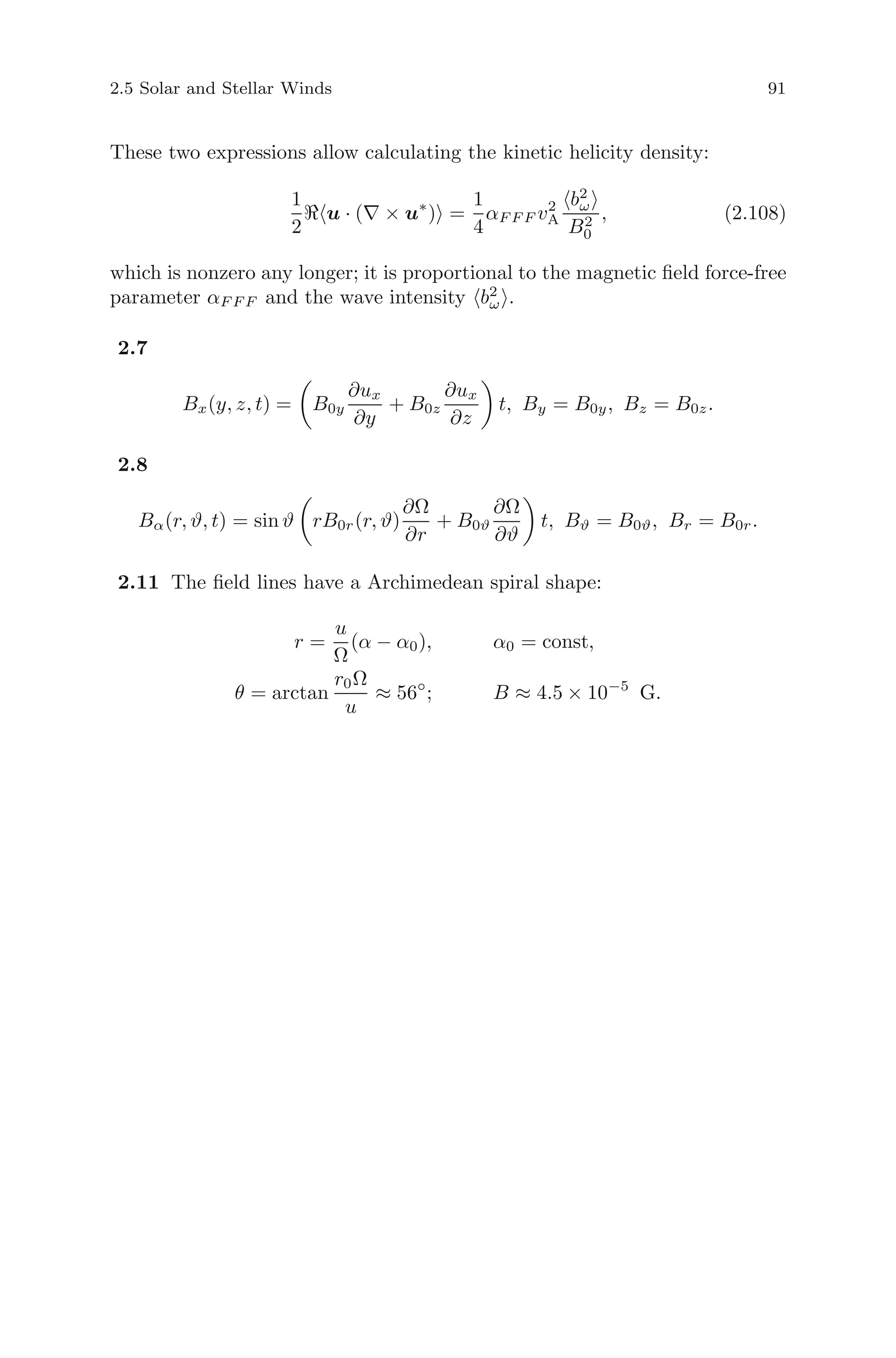
Problems
2.1 Using the Faraday induction law and dissipation-free equations (2.28),
prove that the magnetic flux through arbitrary closed contour remains con-
stant regardless contour motions and deformations.
2.2 Adopt stationary equilibrium of the conducting fluid in a magnetic field.
Demonstrate that the vectors of the magnetic field B and the current density
j are tangent to the surfaces p(r) = const.
2.3 Adopt that electric current J flows along a hot plasma cylinder with
radius a and a nonuniform current density j(r) (z-pinch). Find stationary
solution P(r) for the plasma pressure under the condition that this pressure
is compensated by the magnetic pressure produced by this electric current
itself. Write down a relation linking the total electric current of the pinch
and the pinch pressure integrated over pinch cross section.
Adopt then that the plasma is isothermal and obeys the ideal gas equa-
tion of state [Eq. (2.23)]. Express current J via the plasma temperature T and
the total number of the plasma electrons (or ions) N per unit length of the
cylinder. Calculate the current assuming N ≈ 1015
ions/cm and T ≈ 108
K—
the parameters typical for the nuclear fusion studies; see Fig. 1.1.
2.4 Determine equilibrium condition for the plasma cylinder with radius a, in
which the electric current has only azimuth component jα(r) (so-called theta
pinch). The outside pressure is small and can be discarded compared with the
pinch pressure. Is it possible to ensure equilibrium using some distribution of
the magnetic field produced by external sources?

35. 2.5 Solar and Stellar Winds 87
2.5 The magnetic field is called the force-free field (Sect. 2.3.3) if the density
of Amp`ere’s force is zero everywhere: j × B/c = 0. To ensure this, it is
apparently necessary and sufficient that the electric current is directed along
the field lines everywhere.
(a) Show that the force-free field B satisfies the equation set:
∇ × B = αF F F B, B·∇αF F F = 0,
where αF F F (r) is arbitrary differentiable scalar function (including
constant).
(b) Derive a force-free field dependent on r only in cylindrical coordinates
for αF F F = const.
(c) Is it possible to have a finite energy of the force-free field for αF F F =
const?
(d) Prove that αF F F = const for any force-free field along any field line.
2.6 Consider modification of MHD eigenmodes in a plasma permitted by a
nonpotential force-free magnetic field and calculate the corresponding kinetic
helicity density defined as hk = u(r, t) · ∇ × u(r, t) .
2.7 Adopt that a stationary velocity field u = (ux(y, z), 0, 0) holds in a con-
ducting fluid (shear motion). The initial condition at t = 0 for the magnetic
field is B0 = (0, B0y(y, z), B0z(y, z)). Apply dissipation-free approximation
(νm → ∞) to derive the field at t > 0.
2.8 A stationary differential rotation (i.e., various fluid layer rotate with
different velocities) with an angular velocity Ω = ezΩ(r, ϑ), where r, ϑ are
the spherical coordinates, holds in a conducting fluid. Originally, the mag-
netic field is poloidal, i.e., it belongs to meridian planes: at t = 0, B =
(B0r(r, ϑ), B0ϑ(r, ϑ), 0). Calculate the magnetic field at t > 0 neglecting the
dissipation in the plasma.
2.9 Derive equation (2.98).
2.10 Plot dependences of u and other relevant parameters of the Parker’s
stellar wind on r numerically for different temperature profiles.
2.11 Find the form of interplanetary magnetic field force lines in Parker’s
model (see Sect. 2.5.3). Calculate magnetic field value and the angle θ be-
tween force line and radial direction at the Earth orbit. The solar radius is
a = 0.7 × 106
km; the mean magnetic field at the solar surface B0 ≈ 1 G;
the radius of Earth orbit r0 ≈ 1.5 × 108
km; the angular velocity of solar
rotation Ω = 2.7 × 10−6
rad/s; solar wind velocity u = 300 km/s (slow solar
wind).

36. 88 2 Magnetohydrodynamics of the Cosmic Plasma
2.12 Demonstrate that the solution for the magnetic field in stationary radial
stellar wind (see Sect. 2.5.3) has the form
Br(r, ϑ, α, t) = F α −
(r − a)Ω
u
+ Ωt
a
r
2
2 cosϑ,
Bϑ(r, ϑ, α, t) = p
∂
∂α
F α −
(r − a)Ω
u
+ Ωt
a2
Ω
ur
sin ϑ,
Bα(r, ϑ, α, t) = q F α −
(r − a)Ω
u
+ Ωt
a2
Ω
ur
2 sin ϑ cos ϑ.
Here p and q are constants, which satisfy the condition p+q = 1, and F is an
arbitrary function, specified by the boundary conditions at the solar surface.
Answers and Solutions
2.2 In the static equilibrium (u = 0) and in the absence of non- electro-
magnetic, forces the equilibrium condition reads ∇p = j × B/c. Thus the
vectors B and j are transverse to the pressure gradient and so tangent to
the isobaric surfaces.
2.3 The magnetic field has one component:
Bϕ ≡ B(r) =
4π
cr
r
0
rj(r) dr.
Integrating the equilibrium condition, which follows from Eq. (2.13a) for u = 0
with the boundary condition p r≥a
= 0, we obtain
p (r) =
1
8π
a
r
1
r2
d
dr
(r2
B2
) dr, (1)
where B = (4π/cr)
r
0 rj(r) dr at r < a and B = 2J/cr at r > a. To link
the total current with the pressure we integrate Eq. (1) over full transverse
section and apply the relation aB(a) = 2J/c, which yields
a
0
p (r)2πr dr =
J2
2c2
. (2)
Assuming that the plasma is an equilibrium ideal gas with a given tem-
perature T (in units of energy), we adopt p = 2n(r)T and then Eq. (2) yields
J = 2c
√
NT. (3)

37. 2.5 Solar and Stellar Winds 89
Substitution of required numbers into (3) results in J = 7.5 × 104
A. In prac-
tice the plasma is often non-isothermal, with the electron temperature ex-
ceeding the ion temperature. To maintain the equilibrium the current must
grow in time, because the current results in the increase of both temperature
and pressure. In addition, the pinch can become unstable relative to kink or
sausage mode instabilities.
2.4 The magnetic field inside the cylinder has one component Bz(r) ≡
B(r) = (4π/c)
a
r jϕ(r)dr. The equilibrium inside the cylinder requires con-
stancy of the full pressure:
p (r) +
B2
(r)
8π
= const.
Outside the cylinder without any medium we have p = 0 and the magnetic
field generated by the azimuth current is zero, B = 0; thus, the internal
pressure can only be balanced by a magnetic pressure produced by a field
directed along the cylinder axes, whose value at the side surface of the cylinder
is B0 = 8πp (a). The magnetic field inside the cylinder is always smaller
than the external field:
B2
8π
=
B2
0
8π
− p;
thus, the plasma is a diamagnetic.
2.5 (b) B(r) = B0 ·(0, J1(αF F F r), J0(αF F F r)), where Jn(x) is the Bessel
function.
2.6 To investigate properties of weakly damping linear modes we neglect the
dissipative terms entirely in MHD Eqs. (2.13) and (2.16). Then, for simplicity,
we only consider the helicity originating from the magnetic field twist (the
corresponding pseudoscalar is formed by the dot product of the polar vector
j and the axial vector B: j · B, while no other polar vectors are explicitly
considered) and so we neglect the kinetic pressure and the external force
assuming that their contribution to the helicity is smaller; so the equations
read
∇·B = 0,
∂B
∂t
= ∇ × [u × B], (2.100a)
ρ
∂u
∂t
+ (u·∇)u =
1
4π
[∇ × B] × B. (2.100b)
Now, to describe the small-amplitude linear modes satisfying these equa-
tions, we have to linearize them adopting B = B0 + b for the magnetic field
and adopting b and u to be the first-order oscillating values of an MHD
mode. Importantly, that upon substitution of B = B0 + b into Eq. (2.100b)
we have to take into account that in the nonpotential force-free field ∇×B0 =
αF F F B0 = 0 unlike cases of a uniform field or nonuniform potential field,
which yields

38. 90 2 Magnetohydrodynamics of the Cosmic Plasma
∂b
∂t
= (B0 · ∇)u − (u · ∇)B0,
∂u
∂t
=
αF F F
4πρ
B0 × b +
1
4πρ
(∇ × b) × B0.
(2.101)
Within the eikonal approximation (i.e., adopting the wavelengths of the
eigenmodes to be small compared with the source inhomogeneity scale) we
can write b = bωeiψ(r)−iωt
and a similar for u, which yields equations for the
corresponding complex amplitudes:
b = (i/ω)[i(B0 · ∇ψ)u − (u · ∇)B0], (2.102a)
u =
iαF F F
4πρω
B0 × b −
1
4πρω
[(b · B0)∇ψ − (B0 · ∇ψ)b]. (2.102b)
Let us solve these equations to the first-order accuracy over the small
parameter αF F F /|∇ψ| 1. In the zeroth-order approximation we have
b = −
1
ω
(B0 · ∇ψ)u, u = −
1
4πρω
(B0 · ∇ψ)b, (2.103)
which yields the eikonal
∇ ψ = ±ω/vA, vA = B0/ 4πρ. (2.104)
It is easy to see that in the zeroth approximation these perturbations are
identical to the purely alfv´enic modes for which the conditions b · ∇ψ =
0, u · ∇ψ = 0, b · B0 = 0, and u × b = 0 are satisfied.
Since we use the complex amplitudes, the bilinear terms like ab must
be computed as (1/2) ab∗
, where in addition to averaging over the period
T = 2π/ω we also average over the random phases of Fourier harmonics:
bμb∗
ν = (1/2) b2
ω (δμν − eμeν). (2.105)
In the zeroth over αF F F approximation, the kinetic helicity parameter is
zero: u · (∇ × u∗
) = 0.
Now, taking into account the first order over |αF F F /∇ψ| terms, Eq. (2.102b)
yields
u = −
1
4πρω
(B0 · ∇ψ)b +
1
4πρω
[iαF F F B0 × b + (b · B0)∇ψ], (2.106)
where b · B0 = 0 and
∇ × u = −
i
4πρω
(B0 · ∇ψ)(∇ψ × b)
+
i
4πρω
[−∇ψ × (b · ∇)B0 + b × (B0 · ∇)∇ψ + b × (∇ψ · ∇)B0].
(2.107)

39. 2.5 Solar and Stellar Winds 91
These two expressions allow calculating the kinetic helicity density:
1
2
u · (∇ × u∗
) =
1
4
αF F F v2
A
b2
ω
B2
0
, (2.108)
which is nonzero any longer; it is proportional to the magnetic field force-free
parameter αF F F and the wave intensity b2
ω .
2.7
Bx(y, z, t) = B0y
∂ux
∂y
+ B0z
∂ux
∂z
t, By = B0y, Bz = B0z.
2.8
Bα(r, ϑ, t) = sin ϑ rB0r(r, ϑ)
∂Ω
∂r
+ B0ϑ
∂Ω
∂ϑ
t, Bϑ = B0ϑ, Br = B0r.
2.11 The field lines have a Archimedean spiral shape:
r =
u
Ω
(α − α0), α0 = const,
θ = arctan
r0Ω
u
≈ 56◦
; B ≈ 4.5 × 10−5
G.