Downloaded 24 times
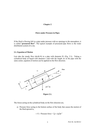

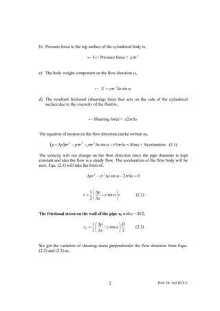
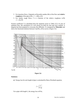
![Prof. Dr. Atıl BULU21
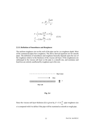
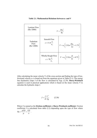
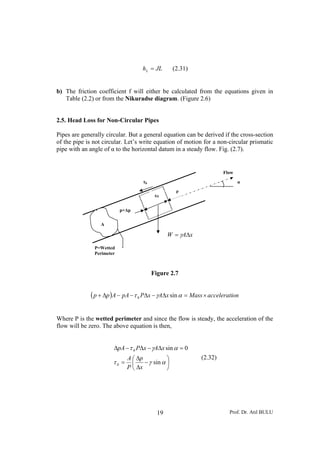
Table 2.3.
Circular Pipes Non-Circular pipes
J
D
4
0 γτ =
g
V
D
f
J
2
2
×=
( )eDff Re,=
υ
VD
=Re
RJγτ =0
g
V
R
f
J
24
2
×=
( )eRff 4Re,=
υ
RV 4
Re =
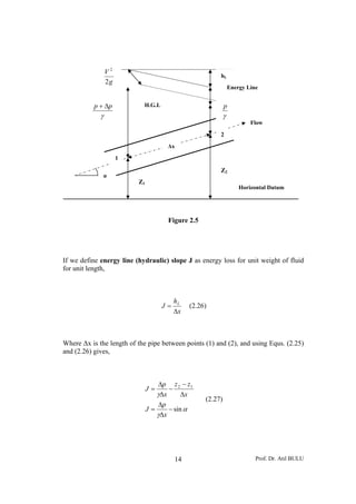
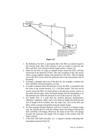
2.6. Hydraulic and Energy Grade Lines
The terms of energy equation have a dimension of length[ ]L ; thus we can attach a
useful relationship to them.
Lhz
g
Vp
z
g
Vp
+++=++ 2
2
22
1
2
11
22 γγ
(2.36)
If we were to tap a piezometer tube into the pipe, the liquid in the pipe would rise in
the tube to a height p/γ (pressure head), hence that is the reason for the name
hydraulic grade line (HGL). The total head ⎟⎟
⎠
⎞
⎜⎜
⎝
⎛
++ z
g
Vp
2
2
γ
in the system is greater
than ⎟⎟
⎠
⎞
⎜⎜
⎝
⎛
+ z
p
γ
by an amount
g
V
2
2
(velocity head), thus the energy (grade) line (EGL)
is above the HGL with a distance
g
V
2
2
.
Some hints for drawing hydraulic grade lines and energy lines are as follows.](https://image.slidesharecdn.com/lecturenotes02-160123205315/85/Flows-under-Pressure-in-Pipes-Lecture-notes-02-21-320.jpg)

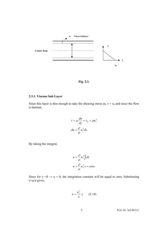
This document discusses fluid flow in pipes under pressure. It presents equations to describe laminar and turbulent flow. For laminar flow, the Hagen-Poiseuille equation gives the relationship between pressure drop and flow rate. For turbulent flow, the velocity profile consists of a thin viscous sublayer near the wall and a fully turbulent center zone. Equations are derived to describe velocity profiles in both the sublayer and center zone based on viscosity and turbulence effects. Pipes are classified as smooth or rough depending on roughness size compared to the sublayer thickness.


