Introduction to Support
Vector Machines
Note to other teachers and users of
these slides. Andrew would be delighted
if you found this source material useful in
giving your own lectures. Feel free to use
these slides verbatim, or to modify them
to fit your own needs. PowerPoint
originals are available. If you make use
of a significant portion of these slides in
your own lecture, please include this
message, or the following link to the
source repository of Andrew’s tutorials:
http://www.cs.cmu.edu/~awm/tutorials .
Comments and corrections gratefully
received.
Thanks:
Andrew Moore
CMU
And
Martin Law
Michigan State University
2023/3/6 2
History of SVM
 SVM is related to statistical learning theory [3]
 SVM was first introduced in 1992 [1]
 SVM becomes popular because of its success in
handwritten digit recognition
 1.1% test error rate for SVM. This is the same as the error
rates of a carefully constructed neural network, LeNet 4.
 See Section 5.11 in [2] or the discussion in [3] for details
 SVM is now regarded as an important example of “kernel
methods”, one of the key area in machine learning
 Note: the meaning of “kernel” is different from the “kernel”
function for Parzen windows
[1] B.E. Boser et al. A Training Algorithm for Optimal Margin Classifiers. Proceedings of the Fifth Annual Workshop on
Computational Learning Theory 5 144-152, Pittsburgh, 1992.
[2] L. Bottou et al. Comparison of classifier methods: a case study in handwritten digit recognition. Proceedings of the 12th
IAPR International Conference on Pattern Recognition, vol. 2, pp. 77-82.
[3] V. Vapnik. The Nature of Statistical Learning Theory. 2nd edition, Springer, 1999.
2023/3/6 3
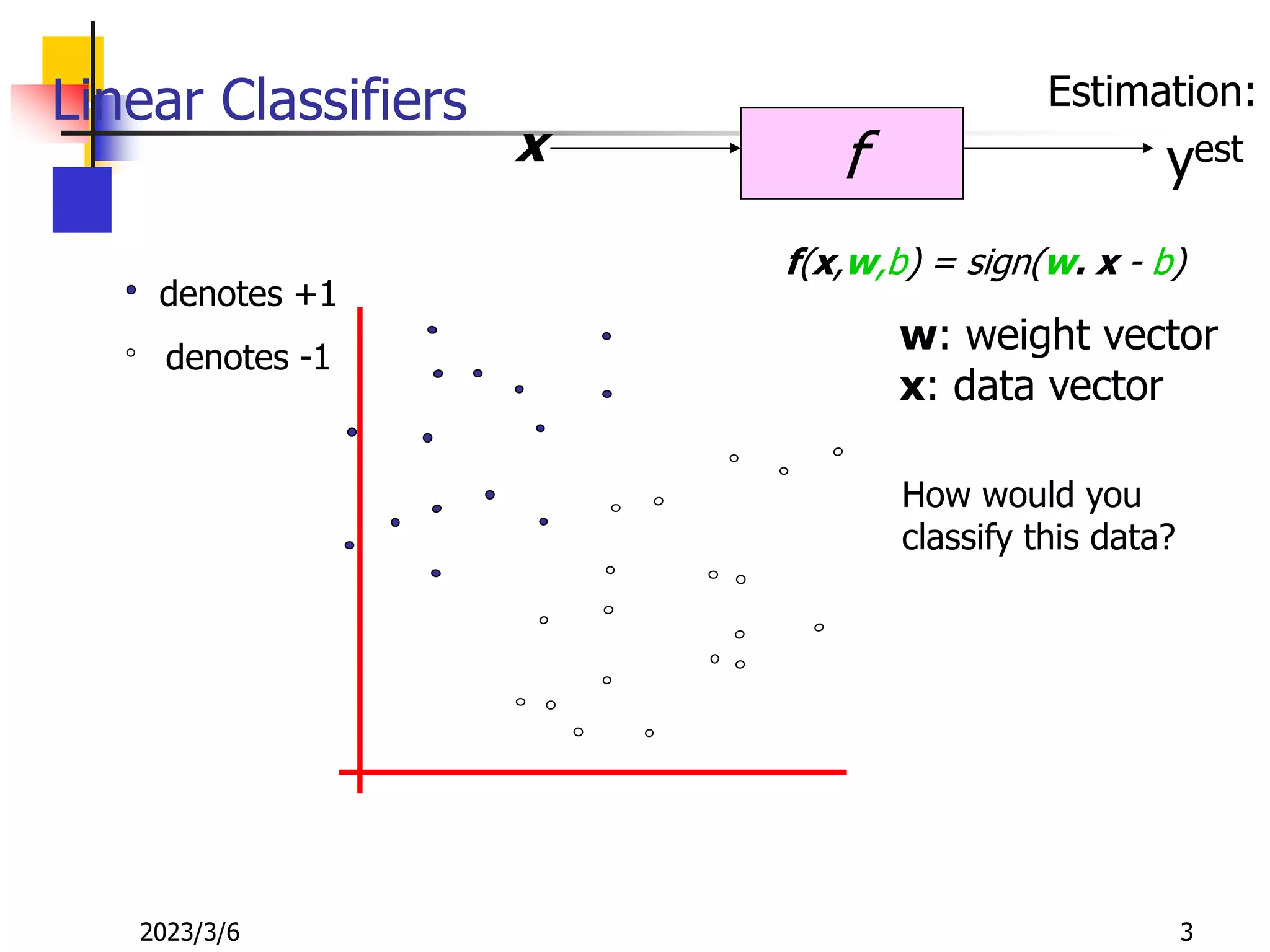
Linear Classifiers
f
x yest
denotes +1
denotes -1
f(x,w,b) = sign(w. x - b)
How would you
classify this data?
Estimation:
w: weight vector
x: data vector
2023/3/6 4
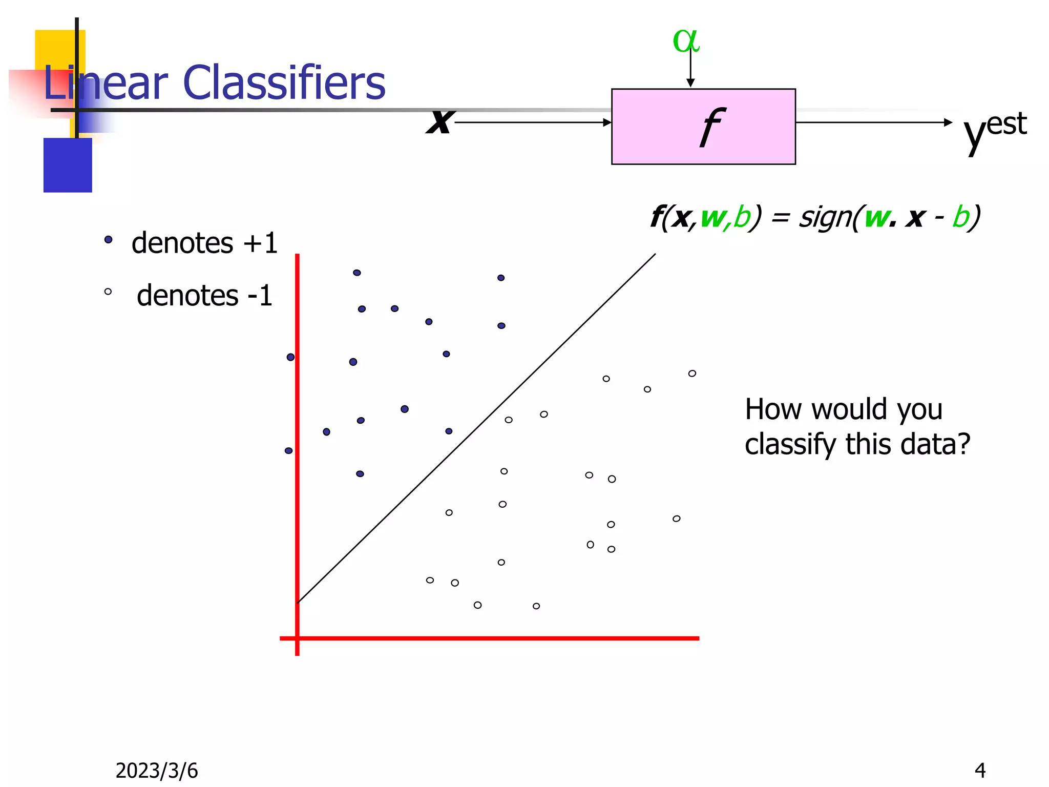
Linear Classifiers
f
x
a
yest
denotes +1
denotes -1
f(x,w,b) = sign(w. x - b)
How would you
classify this data?
2023/3/6 5
Linear Classifiers
f
x
a
yest
denotes +1
denotes -1
f(x,w,b) = sign(w. x - b)
How would you
classify this data?
2023/3/6 6
Linear Classifiers
f
x
a
yest
denotes +1
denotes -1
f(x,w,b) = sign(w. x - b)
How would you
classify this data?
2023/3/6 7
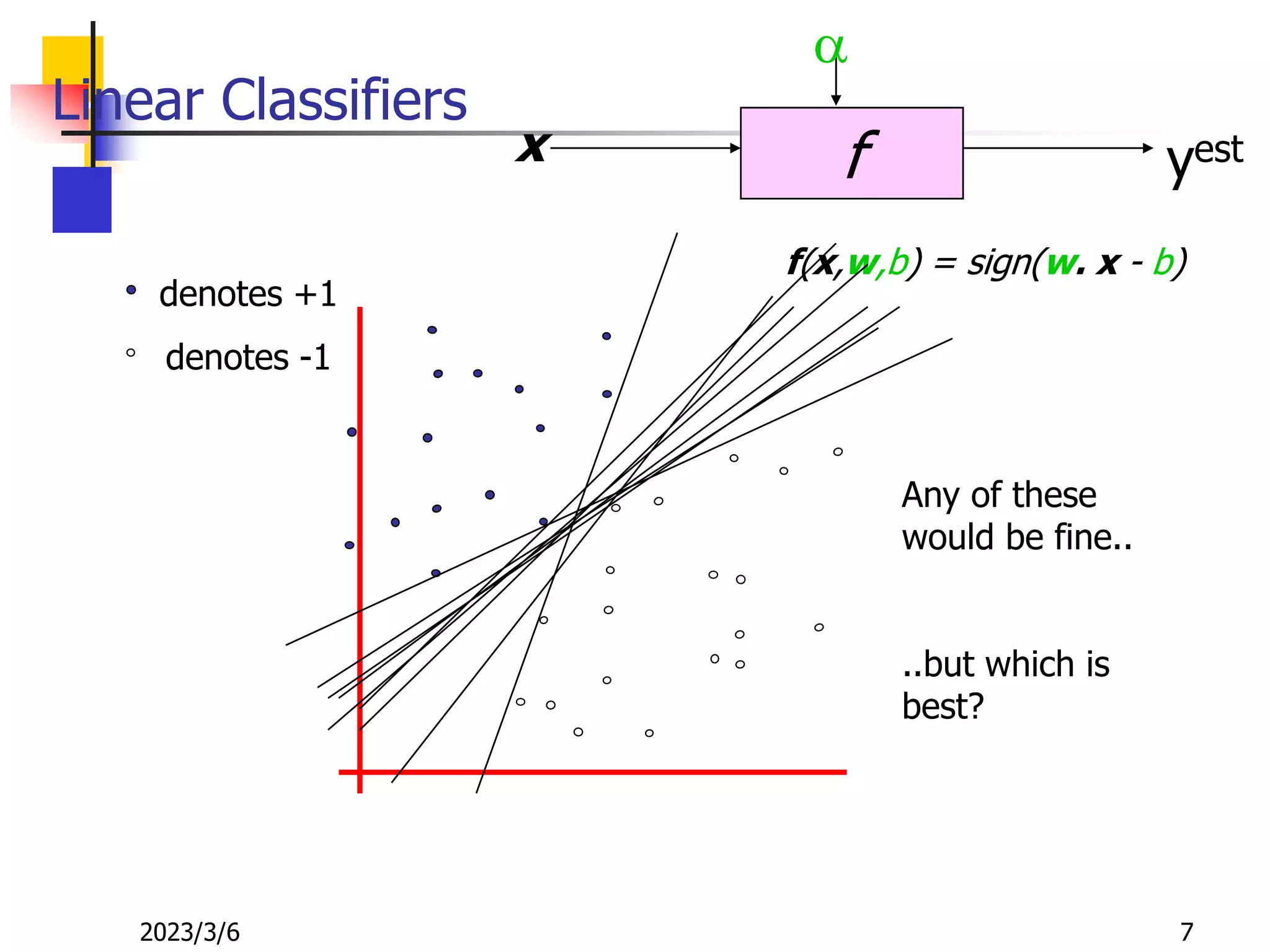
Linear Classifiers
f
x
a
yest
denotes +1
denotes -1
f(x,w,b) = sign(w. x - b)
Any of these
would be fine..
..but which is
best?
2023/3/6 8
Classifier Margin
f
x
a
yest
denotes +1
denotes -1
f(x,w,b) = sign(w. x - b)
Define the margin
of a linear
classifier as the
width that the
boundary could be
increased by
before hitting a
datapoint.
2023/3/6 9
Maximum Margin
f
x
a
yest
denotes +1
denotes -1
f(x,w,b) = sign(w. x - b)
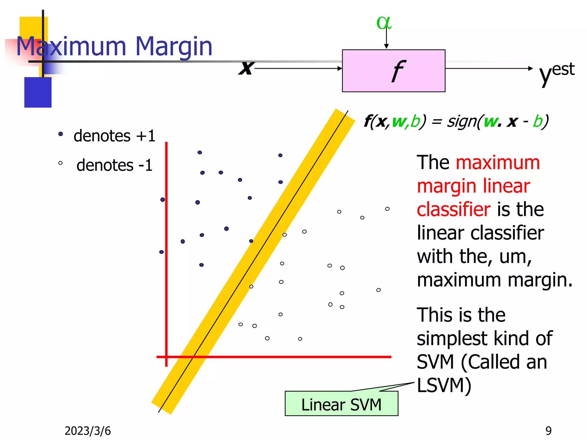
The maximum
margin linear
classifier is the
linear classifier
with the, um,
maximum margin.
This is the
simplest kind of
SVM (Called an
LSVM)
Linear SVM
2023/3/6 10
Maximum Margin
f
x
a
yest
denotes +1
denotes -1
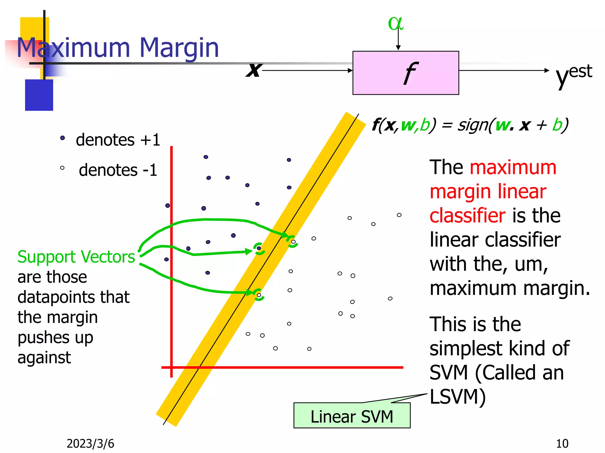
f(x,w,b) = sign(w. x + b)
The maximum
margin linear
classifier is the
linear classifier
with the, um,
maximum margin.
This is the
simplest kind of
SVM (Called an
LSVM)
Support Vectors
are those
datapoints that
the margin
pushes up
against
Linear SVM
2023/3/6 11
Why Maximum Margin?
denotes +1
denotes -1
f(x,w,b) = sign(w. x - b)
The maximum
margin linear
classifier is the
linear classifier
with the, um,
maximum margin.
This is the
simplest kind of
SVM (Called an
LSVM)
Support Vectors
are those
datapoints that
the margin
pushes up
against
2023/3/6 12
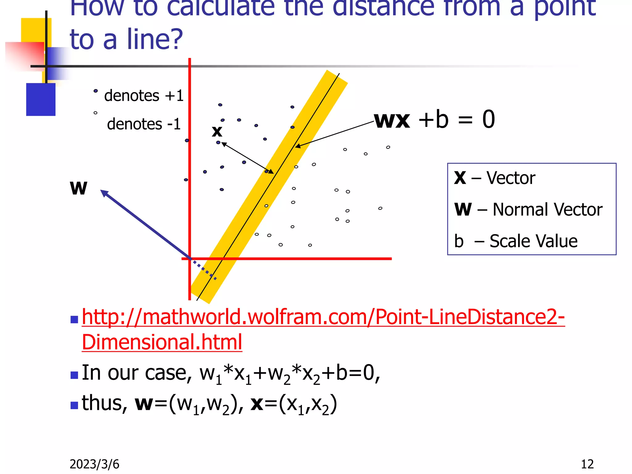
How to calculate the distance from a point
to a line?
 http://mathworld.wolfram.com/Point-LineDistance2-
Dimensional.html
 In our case, w1*x1+w2*x2+b=0,
 thus, w=(w1,w2), x=(x1,x2)
denotes +1
denotes -1 x
wx +b = 0
X – Vector
W – Normal Vector
b – Scale Value
W
2023/3/6 13
Estimate the Margin
 What is the distance expression for a point x to a line
wx+b= 0?
denotes +1
denotes -1 x
wx +b = 0
2 2
1
2
( )
d
i
i
b b
d
w

   
 

x w x w
x
w
X – Vector
W – Normal Vector
b – Scale Value
W
2023/3/6 14
Large-margin Decision Boundary
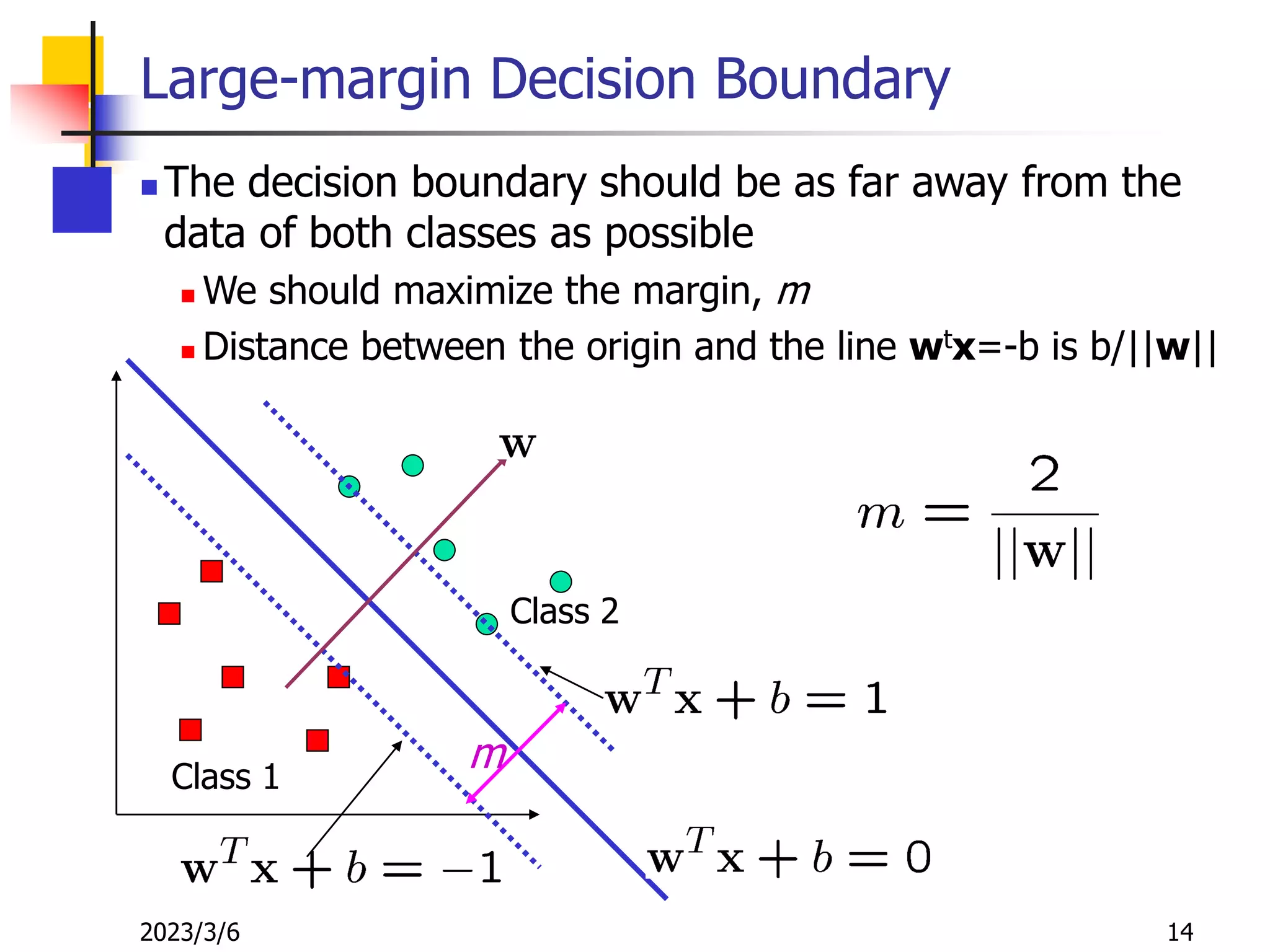
 The decision boundary should be as far away from the
data of both classes as possible
 We should maximize the margin, m
 Distance between the origin and the line wtx=-b is b/||w||
Class 1
Class 2
m
2023/3/6 15
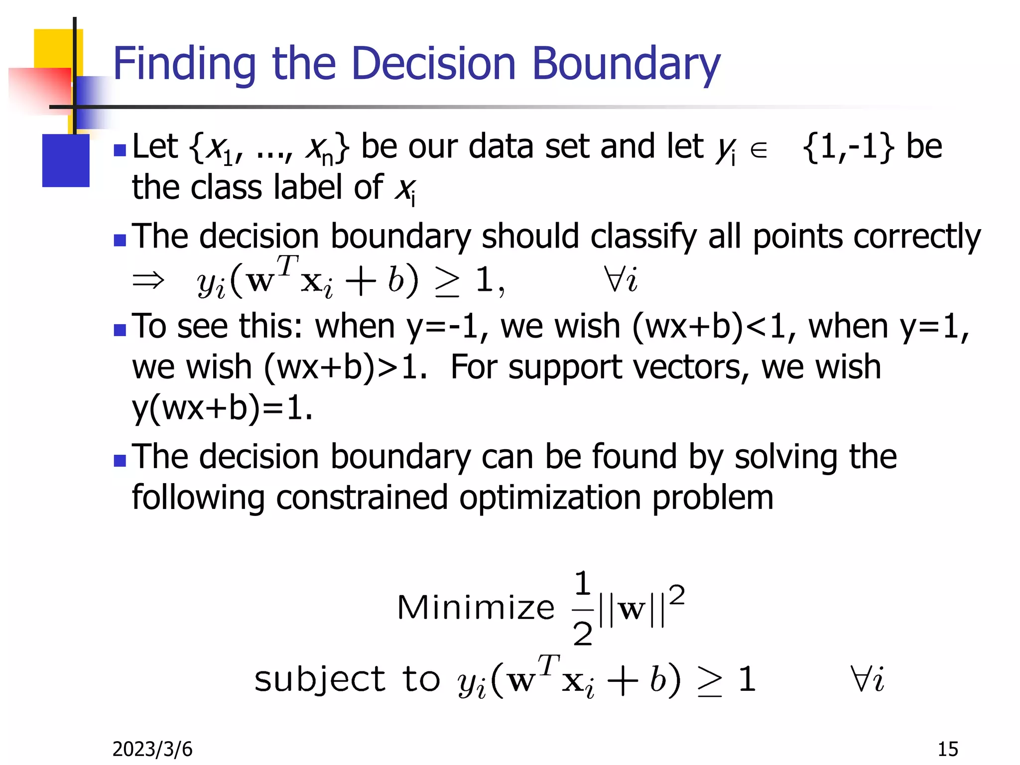
Finding the Decision Boundary
 Let {x1, ..., xn} be our data set and let yi  {1,-1} be
the class label of xi
 The decision boundary should classify all points correctly

 To see this: when y=-1, we wish (wx+b)<1, when y=1,
we wish (wx+b)>1. For support vectors, we wish
y(wx+b)=1.
 The decision boundary can be found by solving the
following constrained optimization problem
2023/3/6 16
Next step… Optional
 Converting SVM to a form we can solve
 Dual form
 Allowing a few errors
 Soft margin
 Allowing nonlinear boundary
 Kernel functions
2023/3/6 17
The Dual Problem (we ignore the derivation)
 The new objective function is in terms of ai only
 It is known as the dual problem: if we know w, we
know all ai; if we know all ai, we know w
 The original problem is known as the primal problem
 The objective function of the dual problem needs to be
maximized!
 The dual problem is therefore:
Properties of ai when we introduce
the Lagrange multipliers
The result when we differentiate the
original Lagrangian w.r.t. b
2023/3/6 18
The Dual Problem
 This is a quadratic programming (QP) problem
 A global maximum of ai can always be found
 w can be recovered by
2023/3/6 19
Characteristics of the Solution
 Many of the ai are zero (see next page for example)
 w is a linear combination of a small number of data points
 This “sparse” representation can be viewed as data
compression as in the construction of knn classifier
 xi with non-zero ai are called support vectors (SV)
 The decision boundary is determined only by the SV
 Let tj (j=1, ..., s) be the indices of the s support vectors. We
can write
 For testing with a new data z
 Compute and
classify z as class 1 if the sum is positive, and class 2
otherwise
 Note: w need not be formed explicitly
2023/3/6 20
a6=1.4
A Geometrical Interpretation
Class 1
Class 2
a1=0.8
a2=0
a3=0
a4=0
a5=0
a7=0
a8=0.6
a9=0
a10=0
2023/3/6 21
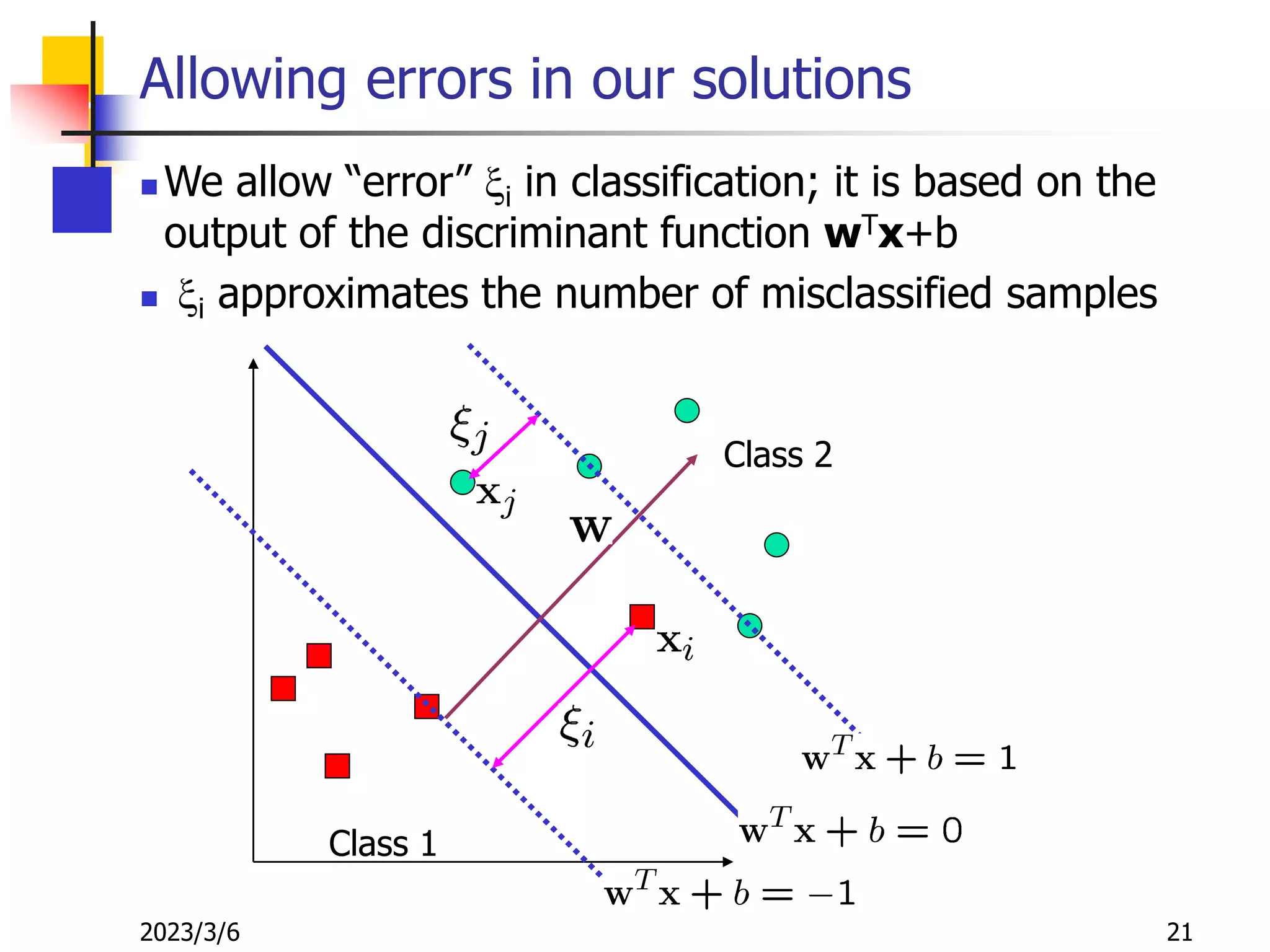
Allowing errors in our solutions
 We allow “error” xi in classification; it is based on the
output of the discriminant function wTx+b
 xi approximates the number of misclassified samples
Class 1
Class 2
2023/3/6 22
Soft Margin Hyperplane
 If we minimize ixi, xi can be computed by
 xi are “slack variables” in optimization
 Note that xi=0 if there is no error for xi
 xi is an upper bound of the number of errors
 We want to minimize
 C : tradeoff parameter between error and margin
 The optimization problem becomes
2023/3/6 23
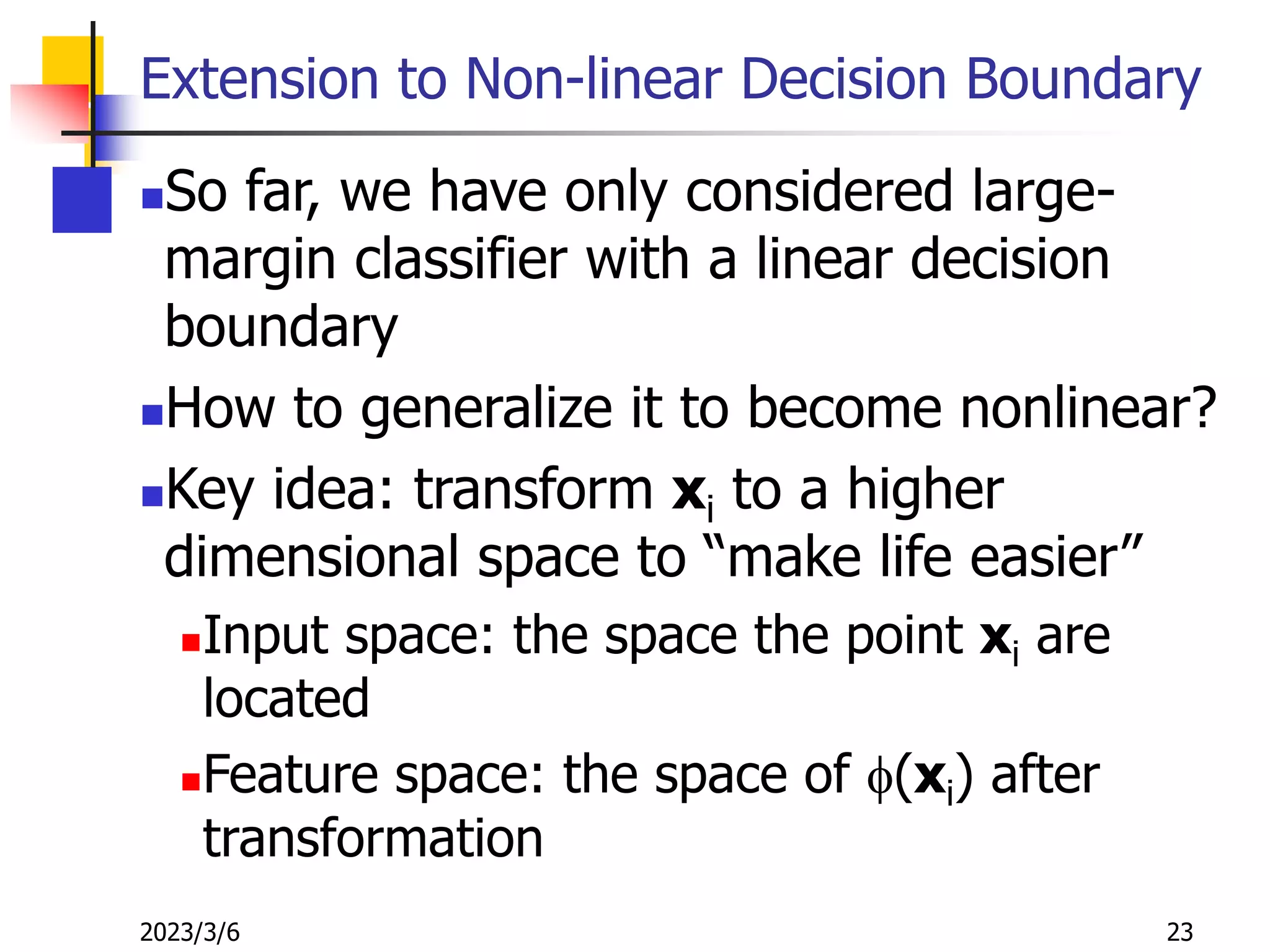
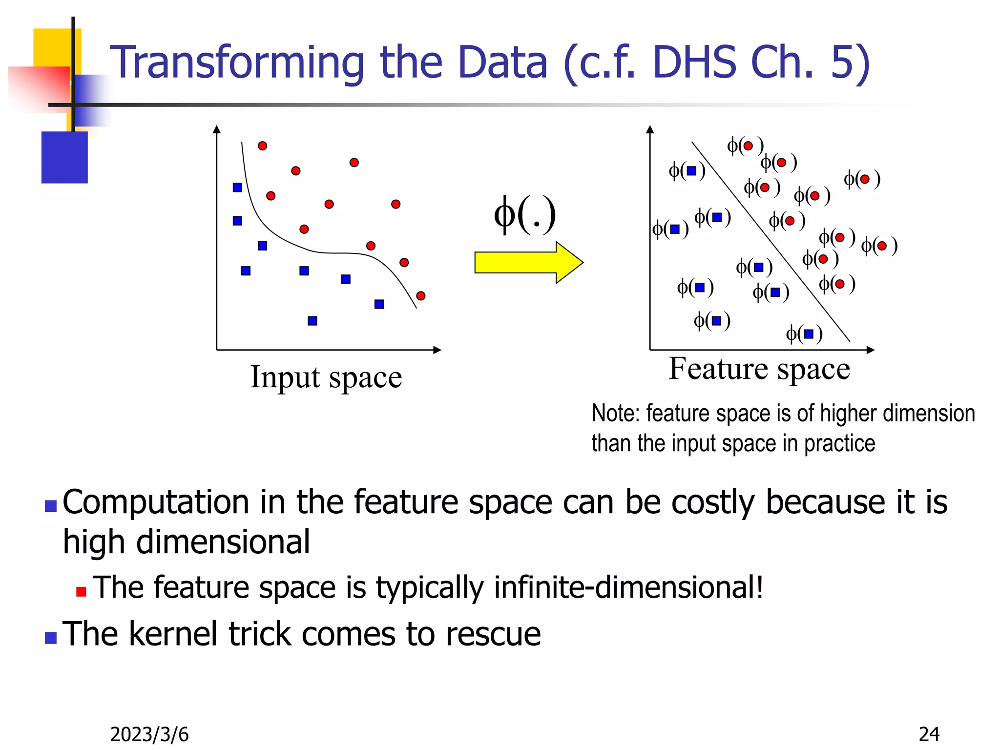
Extension to Non-linear Decision Boundary
So far, we have only considered large-
margin classifier with a linear decision
boundary
How to generalize it to become nonlinear?
Key idea: transform xi to a higher
dimensional space to “make life easier”
Input space: the space the point xi are
located
Feature space: the space of f(xi) after
transformation
2023/3/6 24
Transforming the Data (c.f. DHS Ch. 5)
 Computation in the feature space can be costly because it is
high dimensional
 The feature space is typically infinite-dimensional!
 The kernel trick comes to rescue
f( )
f( )
f( )
f( )
f( )
f( )
f( )
f( )
f(.)
f( )
f( )
f( )
f( )
f( )
f( )
f( )
f( )
f( )
f( )
Feature space
Input space
Note: feature space is of higher dimension
than the input space in practice
2023/3/6 25
The Kernel Trick
 Recall the SVM optimization problem
 The data points only appear as inner product
 As long as we can calculate the inner product in the
feature space, we do not need the mapping explicitly
 Many common geometric operations (angles, distances)
can be expressed by inner products
 Define the kernel function K by
2023/3/6 26
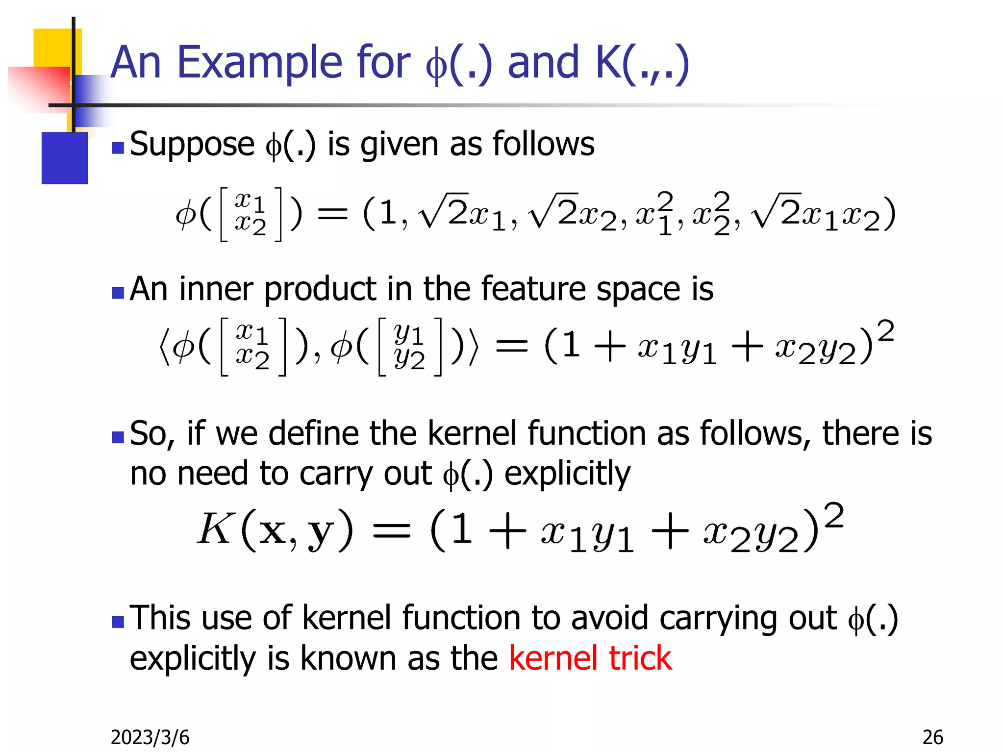
An Example for f(.) and K(.,.)
 Suppose f(.) is given as follows
 An inner product in the feature space is
 So, if we define the kernel function as follows, there is
no need to carry out f(.) explicitly
 This use of kernel function to avoid carrying out f(.)
explicitly is known as the kernel trick
2023/3/6 27
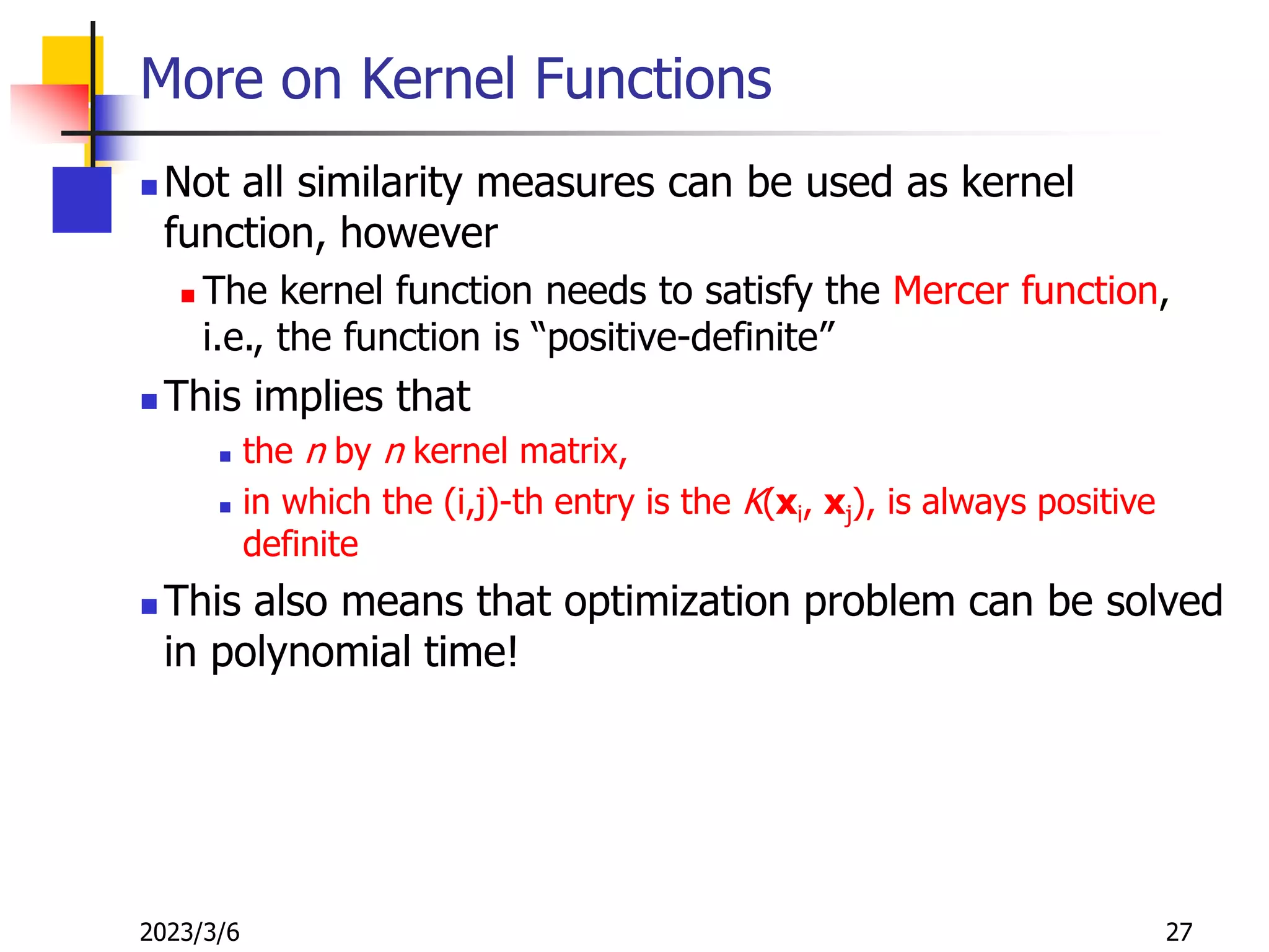
More on Kernel Functions
 Not all similarity measures can be used as kernel
function, however
 The kernel function needs to satisfy the Mercer function,
i.e., the function is “positive-definite”
 This implies that
 the n by n kernel matrix,
 in which the (i,j)-th entry is the K(xi, xj), is always positive
definite
 This also means that optimization problem can be solved
in polynomial time!
2023/3/6 28
Examples of Kernel Functions
 Polynomial kernel with degree d
 Radial basis function kernel with width s
 Closely related to radial basis function neural networks
 The feature space is infinite-dimensional
 Sigmoid with parameter k and q
 It does not satisfy the Mercer condition on all k and q
2023/3/6 29
Non-linear SVMs: Feature spaces
 General idea: the original input space can always be mapped to
some higher-dimensional feature space where the training set is
separable:
Φ: x → φ(x)
2023/3/6 30
Example
 Suppose we have 5 one-dimensional data points
 x1=1, x2=2, x3=4, x4=5, x5=6, with 1, 2, 6 as class 1 and 4,
5 as class 2  y1=1, y2=1, y3=-1, y4=-1, y5=1
 We use the polynomial kernel of degree 2
 K(x,y) = (xy+1)2
 C is set to 100
 We first find ai (i=1, …, 5) by
2023/3/6 31
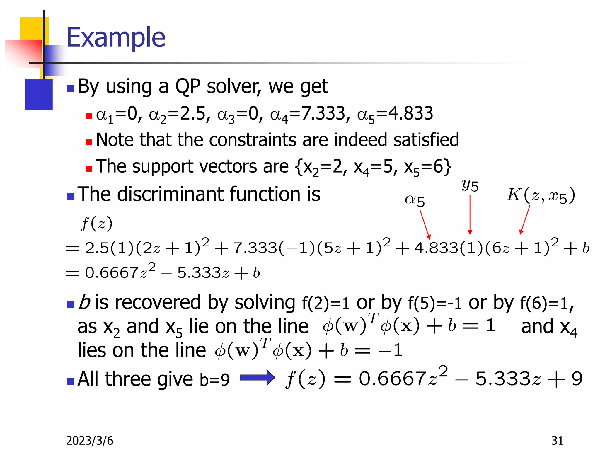
Example
 By using a QP solver, we get
 a1=0, a2=2.5, a3=0, a4=7.333, a5=4.833
 Note that the constraints are indeed satisfied
 The support vectors are {x2=2, x4=5, x5=6}
 The discriminant function is
 b is recovered by solving f(2)=1 or by f(5)=-1 or by f(6)=1,
as x2 and x5 lie on the line and x4
lies on the line
 All three give b=9
2023/3/6 32
Example
Value of discriminant function
1 2 4 5 6
class 2 class 1
class 1
2023/3/6 33
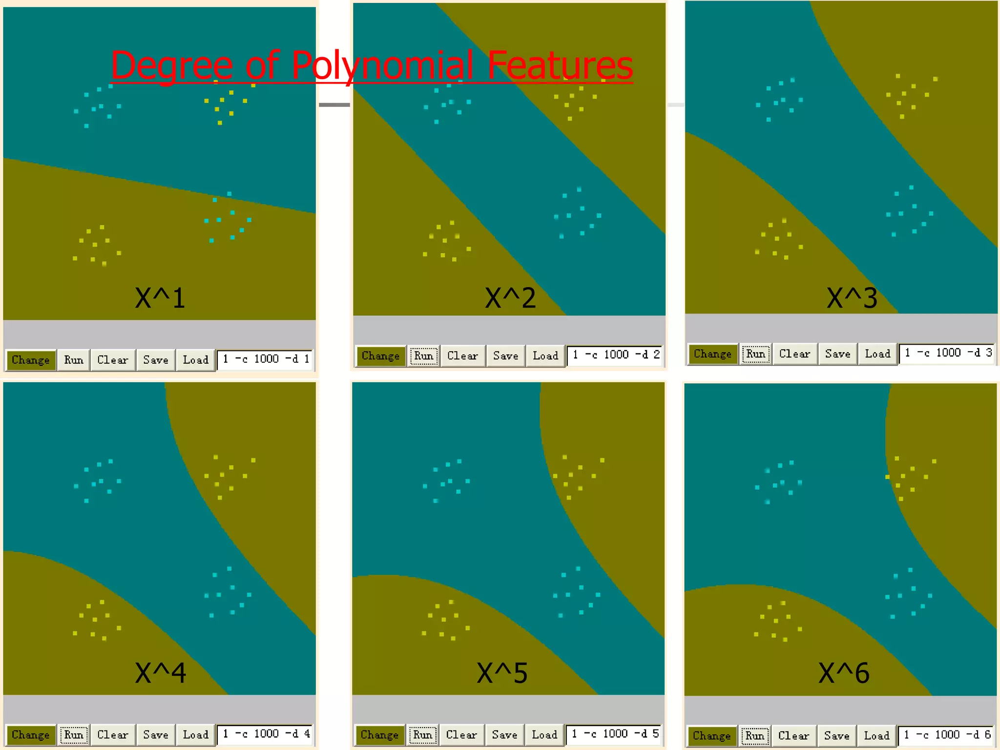
Degree of Polynomial Features
X^1 X^2 X^3
X^4 X^5 X^6
2023/3/6 34
Choosing the Kernel Function
 Probably the most tricky part of using SVM.
2023/3/6 35
Software
 A list of SVM implementation can be found at
http://www.kernel-machines.org/software.html
 Some implementation (such as LIBSVM) can handle
multi-class classification
 SVMLight is among one of the earliest implementation of
SVM
 Several Matlab toolboxes for SVM are also available
2023/3/6 36
Summary: Steps for Classification
 Prepare the pattern matrix
 Select the kernel function to use
 Select the parameter of the kernel function and the
value of C
 You can use the values suggested by the SVM software, or
you can set apart a validation set to determine the values
of the parameter
 Execute the training algorithm and obtain the ai
 Unseen data can be classified using the ai and the
support vectors
2023/3/6 37
Conclusion
 SVM is a useful alternative to neural networks
 Two key concepts of SVM: maximize the margin and the
kernel trick
 Many SVM implementations are available on the web for
you to try on your data set!
2023/3/6 38
Resources
 http://www.kernel-machines.org/
 http://www.support-vector.net/
 http://www.support-vector.net/icml-tutorial.pdf
 http://www.kernel-machines.org/papers/tutorial-
nips.ps.gz
 http://www.clopinet.com/isabelle/Projects/SVM/applist.h
tml
2023/3/6 39
Appendix: Distance from a point to a line
 Equation for the line: let u be a variable, then any point
on the line can be described as:
 P = P1 + u (P2 - P1)
 Let the intersect point be u,
 Then, u can be determined by:
 The two vectors (P2-P1) is orthogonal to P3-u:
 That is,
 (P3-P) dot (P2-P1) =0
 P=P1+u(P2-P1)
 P1=(x1,y1),P2=(x2,y2),P3=(x3,y3) P1
P2
P3
P
2023/3/6 40
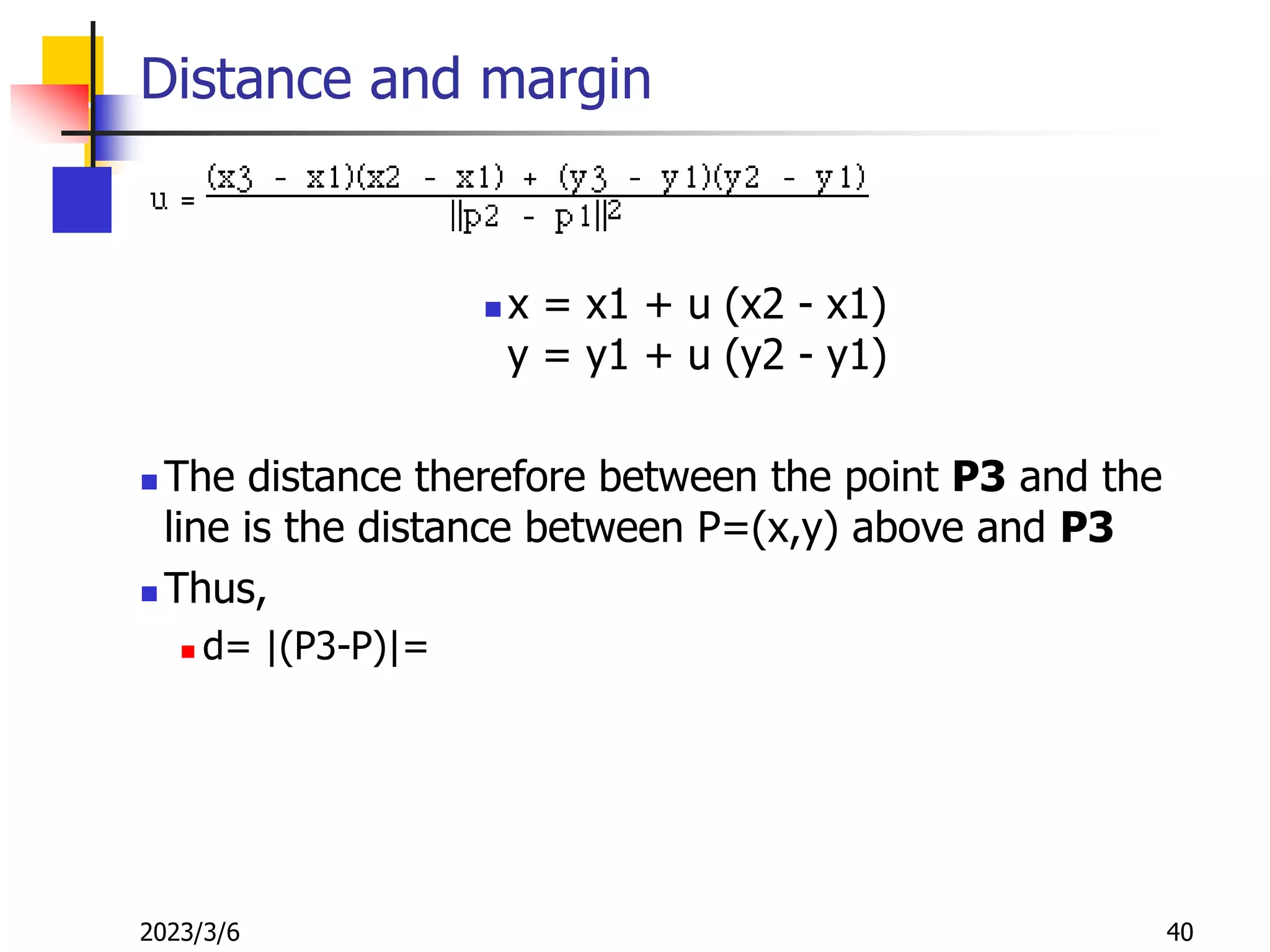
Distance and margin
 x = x1 + u (x2 - x1)
y = y1 + u (y2 - y1)
 The distance therefore between the point P3 and the
line is the distance between P=(x,y) above and P3
 Thus,
 d= |(P3-P)|=

SVM.ppt

  • 1.
    Introduction to Support VectorMachines Note to other teachers and users of these slides. Andrew would be delighted if you found this source material useful in giving your own lectures. Feel free to use these slides verbatim, or to modify them to fit your own needs. PowerPoint originals are available. If you make use of a significant portion of these slides in your own lecture, please include this message, or the following link to the source repository of Andrew’s tutorials: http://www.cs.cmu.edu/~awm/tutorials . Comments and corrections gratefully received. Thanks: Andrew Moore CMU And Martin Law Michigan State University
  • 2.
    2023/3/6 2 History ofSVM  SVM is related to statistical learning theory [3]  SVM was first introduced in 1992 [1]  SVM becomes popular because of its success in handwritten digit recognition  1.1% test error rate for SVM. This is the same as the error rates of a carefully constructed neural network, LeNet 4.  See Section 5.11 in [2] or the discussion in [3] for details  SVM is now regarded as an important example of “kernel methods”, one of the key area in machine learning  Note: the meaning of “kernel” is different from the “kernel” function for Parzen windows [1] B.E. Boser et al. A Training Algorithm for Optimal Margin Classifiers. Proceedings of the Fifth Annual Workshop on Computational Learning Theory 5 144-152, Pittsburgh, 1992. [2] L. Bottou et al. Comparison of classifier methods: a case study in handwritten digit recognition. Proceedings of the 12th IAPR International Conference on Pattern Recognition, vol. 2, pp. 77-82. [3] V. Vapnik. The Nature of Statistical Learning Theory. 2nd edition, Springer, 1999.
  • 3.
    2023/3/6 3 Linear Classifiers f xyest denotes +1 denotes -1 f(x,w,b) = sign(w. x - b) How would you classify this data? Estimation: w: weight vector x: data vector
  • 4.
    2023/3/6 4 Linear Classifiers f x a yest denotes+1 denotes -1 f(x,w,b) = sign(w. x - b) How would you classify this data?
  • 5.
    2023/3/6 5 Linear Classifiers f x a yest denotes+1 denotes -1 f(x,w,b) = sign(w. x - b) How would you classify this data?
  • 6.
    2023/3/6 6 Linear Classifiers f x a yest denotes+1 denotes -1 f(x,w,b) = sign(w. x - b) How would you classify this data?
  • 7.
    2023/3/6 7 Linear Classifiers f x a yest denotes+1 denotes -1 f(x,w,b) = sign(w. x - b) Any of these would be fine.. ..but which is best?
  • 8.
    2023/3/6 8 Classifier Margin f x a yest denotes+1 denotes -1 f(x,w,b) = sign(w. x - b) Define the margin of a linear classifier as the width that the boundary could be increased by before hitting a datapoint.
  • 9.
    2023/3/6 9 Maximum Margin f x a yest denotes+1 denotes -1 f(x,w,b) = sign(w. x - b) The maximum margin linear classifier is the linear classifier with the, um, maximum margin. This is the simplest kind of SVM (Called an LSVM) Linear SVM
  • 10.
    2023/3/6 10 Maximum Margin f x a yest denotes+1 denotes -1 f(x,w,b) = sign(w. x + b) The maximum margin linear classifier is the linear classifier with the, um, maximum margin. This is the simplest kind of SVM (Called an LSVM) Support Vectors are those datapoints that the margin pushes up against Linear SVM
  • 11.
    2023/3/6 11 Why MaximumMargin? denotes +1 denotes -1 f(x,w,b) = sign(w. x - b) The maximum margin linear classifier is the linear classifier with the, um, maximum margin. This is the simplest kind of SVM (Called an LSVM) Support Vectors are those datapoints that the margin pushes up against
  • 12.
    2023/3/6 12 How tocalculate the distance from a point to a line?  http://mathworld.wolfram.com/Point-LineDistance2- Dimensional.html  In our case, w1*x1+w2*x2+b=0,  thus, w=(w1,w2), x=(x1,x2) denotes +1 denotes -1 x wx +b = 0 X – Vector W – Normal Vector b – Scale Value W
  • 13.
    2023/3/6 13 Estimate theMargin  What is the distance expression for a point x to a line wx+b= 0? denotes +1 denotes -1 x wx +b = 0 2 2 1 2 ( ) d i i b b d w         x w x w x w X – Vector W – Normal Vector b – Scale Value W
  • 14.
    2023/3/6 14 Large-margin DecisionBoundary  The decision boundary should be as far away from the data of both classes as possible  We should maximize the margin, m  Distance between the origin and the line wtx=-b is b/||w|| Class 1 Class 2 m
  • 15.
    2023/3/6 15 Finding theDecision Boundary  Let {x1, ..., xn} be our data set and let yi  {1,-1} be the class label of xi  The decision boundary should classify all points correctly   To see this: when y=-1, we wish (wx+b)<1, when y=1, we wish (wx+b)>1. For support vectors, we wish y(wx+b)=1.  The decision boundary can be found by solving the following constrained optimization problem
  • 16.
    2023/3/6 16 Next step…Optional  Converting SVM to a form we can solve  Dual form  Allowing a few errors  Soft margin  Allowing nonlinear boundary  Kernel functions
  • 17.
    2023/3/6 17 The DualProblem (we ignore the derivation)  The new objective function is in terms of ai only  It is known as the dual problem: if we know w, we know all ai; if we know all ai, we know w  The original problem is known as the primal problem  The objective function of the dual problem needs to be maximized!  The dual problem is therefore: Properties of ai when we introduce the Lagrange multipliers The result when we differentiate the original Lagrangian w.r.t. b
  • 18.
    2023/3/6 18 The DualProblem  This is a quadratic programming (QP) problem  A global maximum of ai can always be found  w can be recovered by
  • 19.
    2023/3/6 19 Characteristics ofthe Solution  Many of the ai are zero (see next page for example)  w is a linear combination of a small number of data points  This “sparse” representation can be viewed as data compression as in the construction of knn classifier  xi with non-zero ai are called support vectors (SV)  The decision boundary is determined only by the SV  Let tj (j=1, ..., s) be the indices of the s support vectors. We can write  For testing with a new data z  Compute and classify z as class 1 if the sum is positive, and class 2 otherwise  Note: w need not be formed explicitly
  • 20.
    2023/3/6 20 a6=1.4 A GeometricalInterpretation Class 1 Class 2 a1=0.8 a2=0 a3=0 a4=0 a5=0 a7=0 a8=0.6 a9=0 a10=0
  • 21.
    2023/3/6 21 Allowing errorsin our solutions  We allow “error” xi in classification; it is based on the output of the discriminant function wTx+b  xi approximates the number of misclassified samples Class 1 Class 2
  • 22.
    2023/3/6 22 Soft MarginHyperplane  If we minimize ixi, xi can be computed by  xi are “slack variables” in optimization  Note that xi=0 if there is no error for xi  xi is an upper bound of the number of errors  We want to minimize  C : tradeoff parameter between error and margin  The optimization problem becomes
  • 23.
    2023/3/6 23 Extension toNon-linear Decision Boundary So far, we have only considered large- margin classifier with a linear decision boundary How to generalize it to become nonlinear? Key idea: transform xi to a higher dimensional space to “make life easier” Input space: the space the point xi are located Feature space: the space of f(xi) after transformation
  • 24.
    2023/3/6 24 Transforming theData (c.f. DHS Ch. 5)  Computation in the feature space can be costly because it is high dimensional  The feature space is typically infinite-dimensional!  The kernel trick comes to rescue f( ) f( ) f( ) f( ) f( ) f( ) f( ) f( ) f(.) f( ) f( ) f( ) f( ) f( ) f( ) f( ) f( ) f( ) f( ) Feature space Input space Note: feature space is of higher dimension than the input space in practice
  • 25.
    2023/3/6 25 The KernelTrick  Recall the SVM optimization problem  The data points only appear as inner product  As long as we can calculate the inner product in the feature space, we do not need the mapping explicitly  Many common geometric operations (angles, distances) can be expressed by inner products  Define the kernel function K by
  • 26.
    2023/3/6 26 An Examplefor f(.) and K(.,.)  Suppose f(.) is given as follows  An inner product in the feature space is  So, if we define the kernel function as follows, there is no need to carry out f(.) explicitly  This use of kernel function to avoid carrying out f(.) explicitly is known as the kernel trick
  • 27.
    2023/3/6 27 More onKernel Functions  Not all similarity measures can be used as kernel function, however  The kernel function needs to satisfy the Mercer function, i.e., the function is “positive-definite”  This implies that  the n by n kernel matrix,  in which the (i,j)-th entry is the K(xi, xj), is always positive definite  This also means that optimization problem can be solved in polynomial time!
  • 28.
    2023/3/6 28 Examples ofKernel Functions  Polynomial kernel with degree d  Radial basis function kernel with width s  Closely related to radial basis function neural networks  The feature space is infinite-dimensional  Sigmoid with parameter k and q  It does not satisfy the Mercer condition on all k and q
  • 29.
    2023/3/6 29 Non-linear SVMs:Feature spaces  General idea: the original input space can always be mapped to some higher-dimensional feature space where the training set is separable: Φ: x → φ(x)
  • 30.
    2023/3/6 30 Example  Supposewe have 5 one-dimensional data points  x1=1, x2=2, x3=4, x4=5, x5=6, with 1, 2, 6 as class 1 and 4, 5 as class 2  y1=1, y2=1, y3=-1, y4=-1, y5=1  We use the polynomial kernel of degree 2  K(x,y) = (xy+1)2  C is set to 100  We first find ai (i=1, …, 5) by
  • 31.
    2023/3/6 31 Example  Byusing a QP solver, we get  a1=0, a2=2.5, a3=0, a4=7.333, a5=4.833  Note that the constraints are indeed satisfied  The support vectors are {x2=2, x4=5, x5=6}  The discriminant function is  b is recovered by solving f(2)=1 or by f(5)=-1 or by f(6)=1, as x2 and x5 lie on the line and x4 lies on the line  All three give b=9
  • 32.
    2023/3/6 32 Example Value ofdiscriminant function 1 2 4 5 6 class 2 class 1 class 1
  • 33.
    2023/3/6 33 Degree ofPolynomial Features X^1 X^2 X^3 X^4 X^5 X^6
  • 34.
    2023/3/6 34 Choosing theKernel Function  Probably the most tricky part of using SVM.
  • 35.
    2023/3/6 35 Software  Alist of SVM implementation can be found at http://www.kernel-machines.org/software.html  Some implementation (such as LIBSVM) can handle multi-class classification  SVMLight is among one of the earliest implementation of SVM  Several Matlab toolboxes for SVM are also available
  • 36.
    2023/3/6 36 Summary: Stepsfor Classification  Prepare the pattern matrix  Select the kernel function to use  Select the parameter of the kernel function and the value of C  You can use the values suggested by the SVM software, or you can set apart a validation set to determine the values of the parameter  Execute the training algorithm and obtain the ai  Unseen data can be classified using the ai and the support vectors
  • 37.
    2023/3/6 37 Conclusion  SVMis a useful alternative to neural networks  Two key concepts of SVM: maximize the margin and the kernel trick  Many SVM implementations are available on the web for you to try on your data set!
  • 38.
    2023/3/6 38 Resources  http://www.kernel-machines.org/ http://www.support-vector.net/  http://www.support-vector.net/icml-tutorial.pdf  http://www.kernel-machines.org/papers/tutorial- nips.ps.gz  http://www.clopinet.com/isabelle/Projects/SVM/applist.h tml
  • 39.
    2023/3/6 39 Appendix: Distancefrom a point to a line  Equation for the line: let u be a variable, then any point on the line can be described as:  P = P1 + u (P2 - P1)  Let the intersect point be u,  Then, u can be determined by:  The two vectors (P2-P1) is orthogonal to P3-u:  That is,  (P3-P) dot (P2-P1) =0  P=P1+u(P2-P1)  P1=(x1,y1),P2=(x2,y2),P3=(x3,y3) P1 P2 P3 P
  • 40.
    2023/3/6 40 Distance andmargin  x = x1 + u (x2 - x1) y = y1 + u (y2 - y1)  The distance therefore between the point P3 and the line is the distance between P=(x,y) above and P3  Thus,  d= |(P3-P)|=