Downloaded 22 times
![F (x) =sgn( )
a. The Behaviour of the Sigmoid Kernel
We consider the sigmoid kernel K(xi, xj ) = tanh(axi
T
xj + r), which takes two parameters: a
and r. For a > 0, we can view a as a scaling parameter of the input data, and r as a shifting
parameter that controls the threshold of mapping. For a < 0, the dot-product of the input data
is not only scaled but reversed.
It concludes that the first case, a > 0 and r < 0, is moresuitable for the sigmoid kernel.
A R Results
+ - K is CPD after r is small; similar to RBF for small a
+ + in general not as good as the (+, −) case
- + objective value of (6) −∞ after r large enough
- - easily the objective value of (6) −∞
Table 1: behaviour in different parameter combinations in sigmoid kernel
b. Behaviour of polynomial kernel
Polynomial Kernel (K(xi , xj ) = (1 + xi
T
xj )p
) is non-stochastic kernel estimate with two
parameters i.e. C and polynomial degree p. Each data from the set xi has an influence on
the kernel point of the test value xj, irrespective of its the actual distance from xj [14], It
gives good classification accuracy with minimum number of support vectors and low
classification error.
.
Figure: The effect of the degree of a polynomial kernel.](https://image.slidesharecdn.com/docfile-150127050940-conversion-gate01/75/Introduction-to-Support-Vector-Machines-6-2048.jpg)
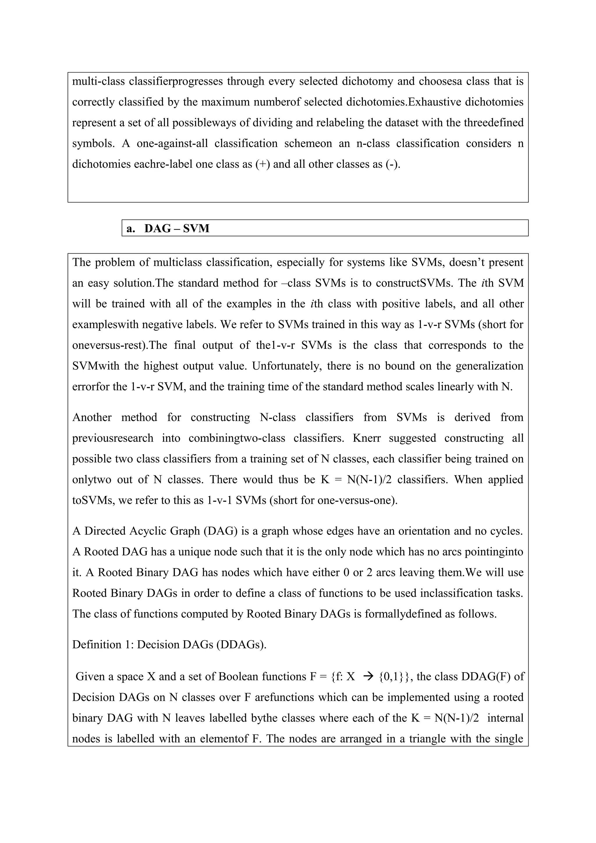
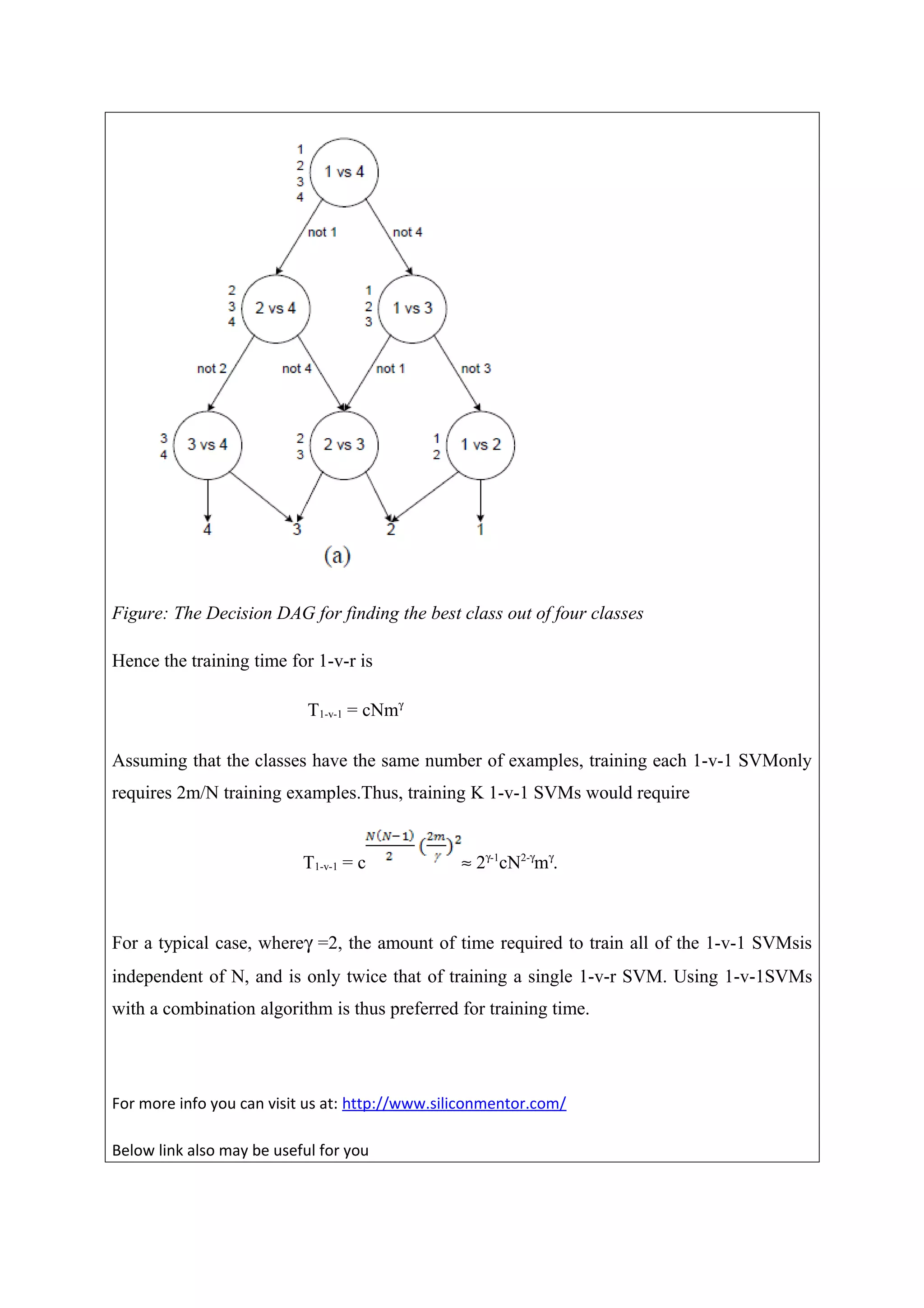
![root node at the top, two nodesin the second layer andso on until the finallayer of N leaves.
The i-th node in layer j<N is connected to the i-th and (i+1)-st node in the (j+1)-st layer.
To evaluate a particular DDAG on input x ∈X, starting at the root node, the binaryfunction at
a node is evaluated. The node is then exited via the left edge, if the binaryfunction is zero; or
the right edge, if the binary function is one. The next node’s binaryfunction is then evaluated.
The value of the decision function D(x) is the value associatedwith the final leaf node. The
path taken through the DDAG is knownas the evaluation path. The input x reaches a node of
the graph, if that node is on theevaluation path for x. We refer to the decision node
distinguishing classes i and j as the ij-node. Assuming that the number of a leaf is its class,
this node is the i-th node in the (N-j+1)-th layer provided i<j. Similarly the j-nodes are those
nodes involving class j, that is, the internal nodes on the two diagonals containing the leaf
labelled by j.
The DDAG is equivalent to operating on a list, where each node eliminates one class fromthe
list. The list is initialized with a list of all classes. A test point is evaluated against thedecision
node that corresponds to the first and last elements of the list.
If the node prefersone of the two classes, the other class is eliminated from the list, and the
DDAG proceedsto test the first and last elements of the new list. The DDAG terminates when
only oneclass remains in the list. Thus, for a problem with N classes, N-1 decision nodes will
beevaluated in order to derive an answer.
The current state of the list is the total state of the system. Therefore, since a list stateis
reachable in more than one possible path through the system, the decision graph thealgorithm
traverses is a DAG, not simply a tree.
The DAGSVM [8] separates the individual classes with large margin. It is safe to discard
thelosing class at each 1-v-1 decision because, for the hard margin case, all of the examplesof
the losing class are far away from the decision surface. The DAGSVM algorithm is superior
to other multiclass SVM algorithms in both trainingand evaluationtime. Empirically,SVM
training is observedto scale super-linearlywith the training set size, according to a power law:
T = cmγ
, whereγ≈2 for algorithmsbasedon the decompositionmethod,with some
proportionalityconstant c. For the standard1-v-r multiclass SVM training algorithm, the entire
training set is used to create all N classifiers.](https://image.slidesharecdn.com/docfile-150127050940-conversion-gate01/75/Introduction-to-Support-Vector-Machines-10-2048.jpg)


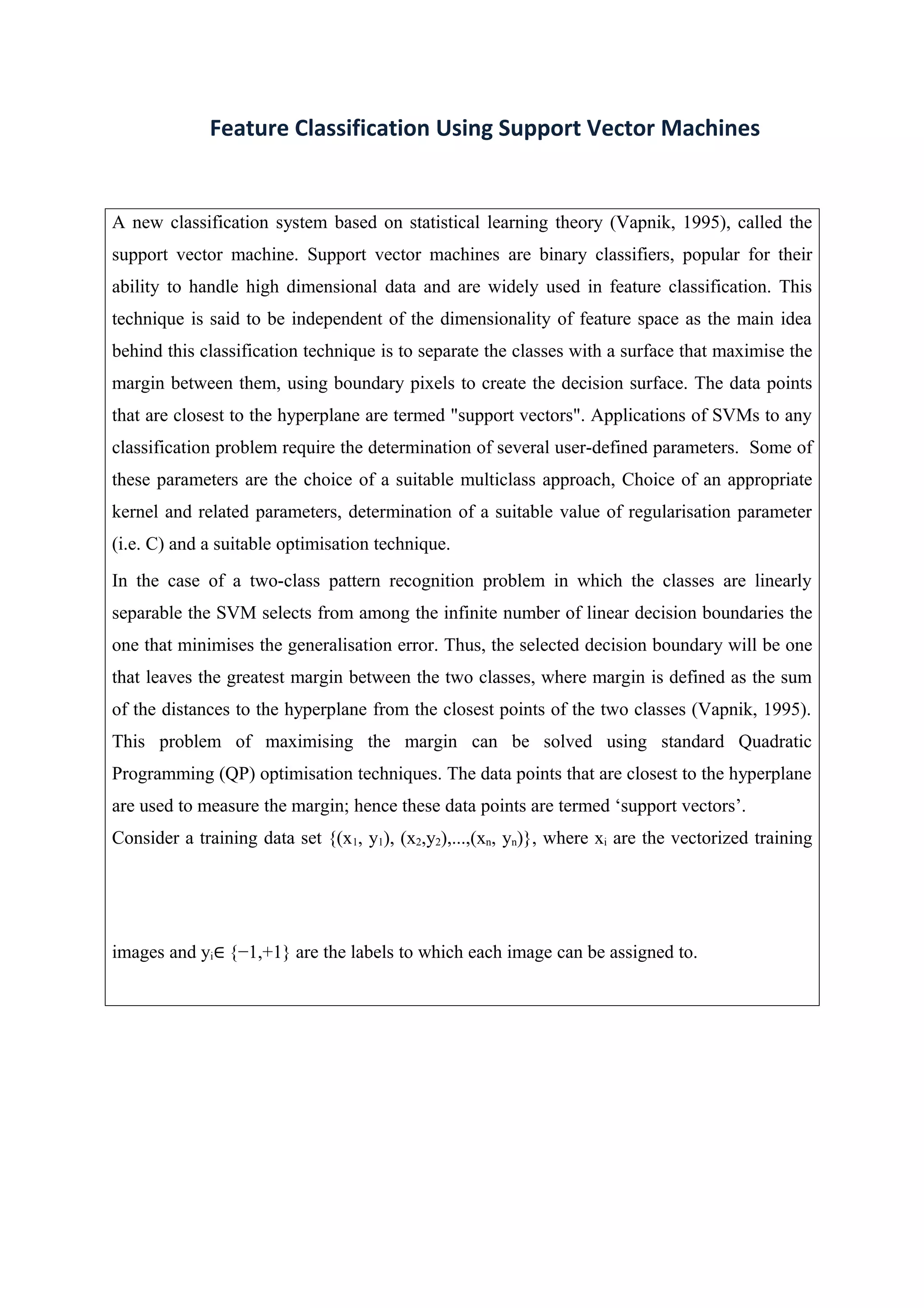
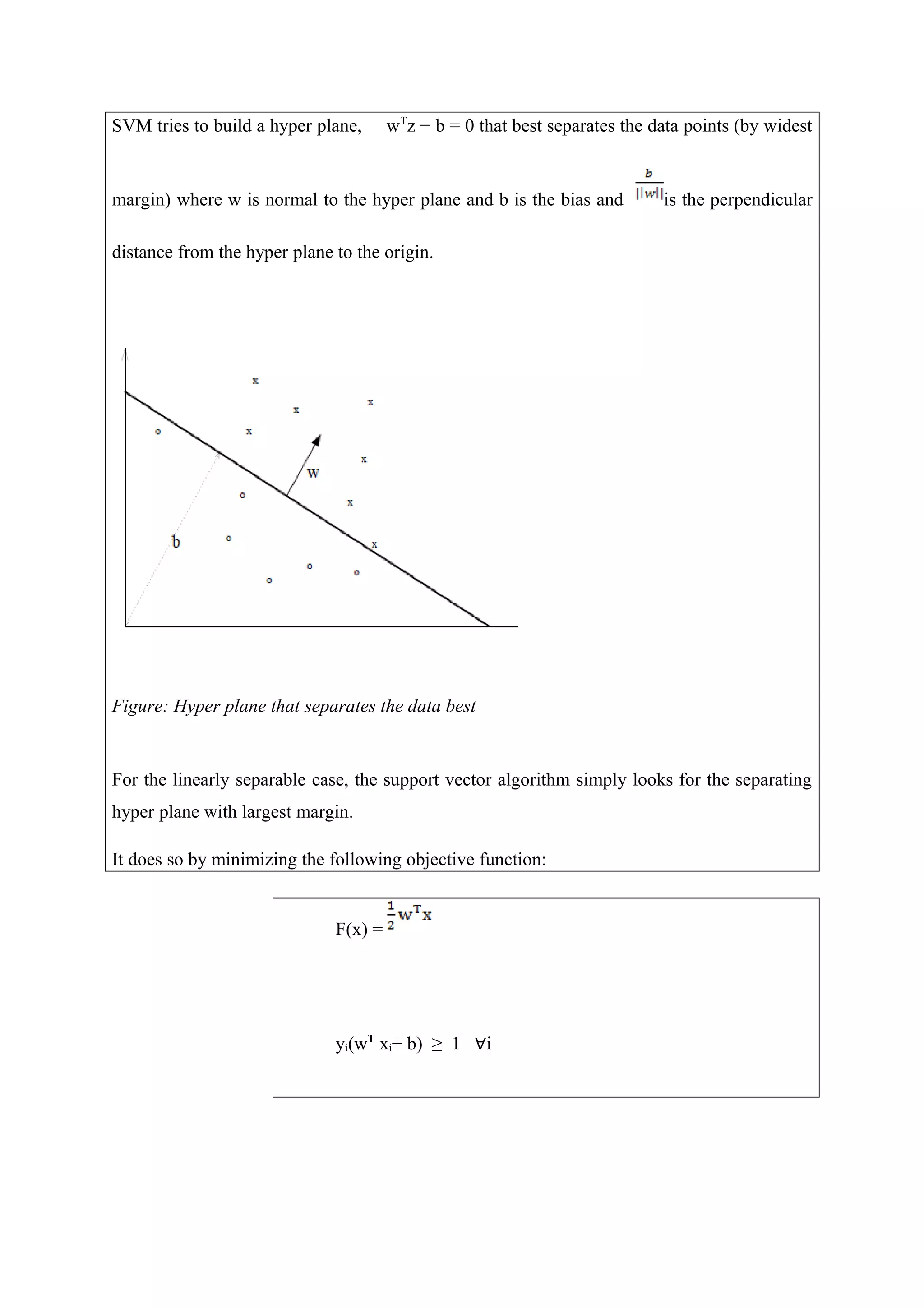
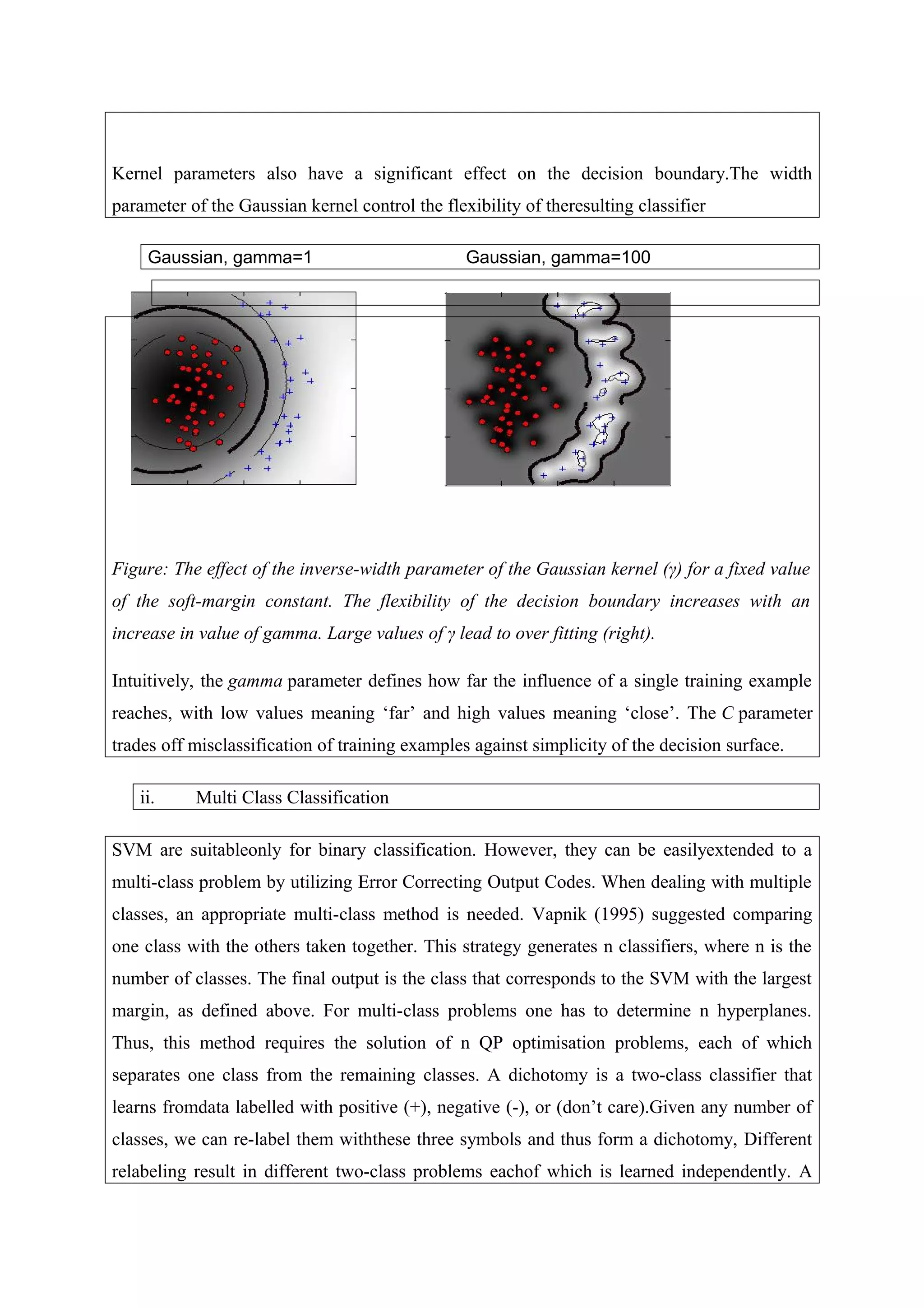
The document discusses the use of Support Vector Machines (SVMs) in feature classification, emphasizing their ability to efficiently handle high dimensional data by maximizing the margin between classes. It explains the underlying statistical learning theory, optimization techniques, and various kernel functions that enhance SVMs for both linear and non-linear classification tasks. Additionally, it covers multi-class classification methods, including one-versus-one and one-versus-rest approaches, highlighting the DAG-SVM as an effective solution for this complexity.