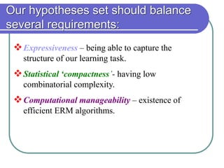
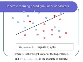
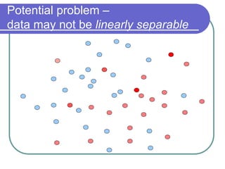
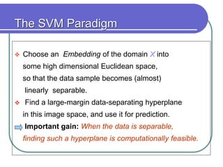
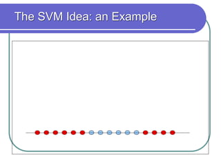
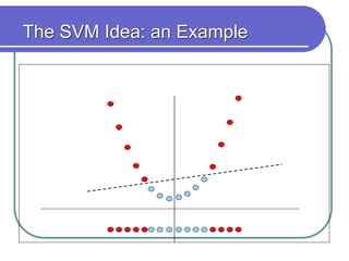
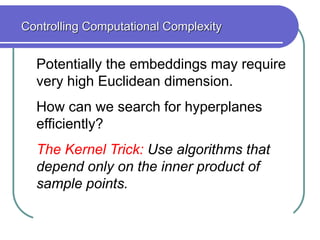
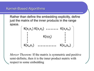
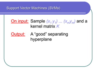
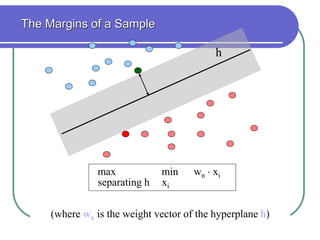
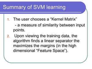
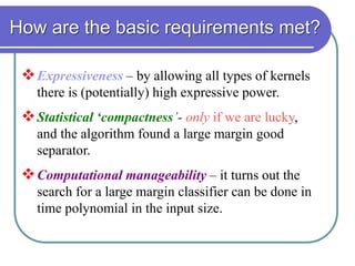
Statistical machine learning aims to develop algorithms that can detect meaningful patterns in large, complex datasets. It focuses on tasks like classification, clustering, and prediction. Support vector machines (SVMs) are a common approach that learns by finding a hyperplane that maximizes the margin between examples of separate classes. SVMs map data into a high-dimensional feature space to allow for linear separation. The kernel trick allows efficient learning without explicitly computing the mapping, by defining a kernel function measuring similarity. SVMs balance expressiveness, statistical soundness, and computational feasibility.

1. Statistical Machine Learning-
The Basic Approach and
Current Research Challenges
Shai Ben-David
CS497
February, 2007

2. A High Level Agenda
“The purpose of science is
to find meaningful simplicity
in the midst of disorderly complexity”
Herbert Simon

3. Representative learning tasks
 Medical research.
 Detection of fraudulent activity
(credit card transactions, intrusion
detection, stock market manipulation)
 Analysis of genome functionality
 Email spam detection.
 Spatial prediction of landslide hazards.

4. Common to all such tasks
 We wish to develop algorithms that detect meaningful
regularities in large complex data sets.
 We focus on data that is too complex for humans to
figure out its meaningful regularities.
 We consider the task of finding such regularities from
random samples of the data population.
 We should derive conclusions in timely manner.
Computational efficiency is essential.

5. Different types of learning tasks
 Classification prediction –
we wish to classify data points into categories, and we
are given already classified samples as our training
input.
For example:
 Training a spam filter
 Medical Diagnosis (Patient info → High/Low risk).
 Stock market prediction ( Predict tomorrow’s market
trend from companies performance data)

6. Other Learning Tasks
 Clustering –
the grouping data into representative collections
- a fundamental tool for data analysis.
Examples :
 Clustering customers for targeted marketing.
 Clustering pixels to detect objects in images.
 Clustering web pages for content similarity.

7. Differences from Classical Statistics
 We are interested in hypothesis generation
rather than hypothesis testing.
 We wish to make no prior assumptions
about the structure of our data.
 We develop algorithms for automated
generation of hypotheses.
 We are concerned with computational
efficiency.

8. Learning Theory:
The fundamental dilemma…
X
Y
y=f(x)
Good models
should enable
Prediction
of new data…
Tradeoff between
accuracy and simplicity

9. A Fundamental Dilemma of Science:
Model Complexity vs Prediction Accuracy
Complexity
Accuracy
Possible
Models/representations
Limited data

12. Problem Outline
 We are interested in
(automated) Hypothesis Generation,
rather than traditional Hypothesis Testing
 First obstacle: The danger of overfitting.
 First solution:
Consider only a limited set of candidate hypotheses.

13. Empirical Risk Minimization
Paradigm
 Choose a Hypothesis Class H of subsets of X.
 For an input sample S, find some h in H that fits S
well.
 For a new point x, predict a label according to its
membership in h.

14. The Mathematical Justification
Assume both a training sample S and the test point
(x,l) are generated i.i.d. by the same distribution over
X x {0,1} then,
If H is not too rich ( in some formal sense) then,
for every h in H, the training error of h on the
sample S is a good estimate of its probability of
success on the new x .
In other words – there is no overfitting

15. Training error
Expected test error
The Mathematical Justification - Formally
|
|
)
1
ln(
)
dim(
|
|
|
}
)
(
:
y)
{(x,
|
)
)
(
(
Pr )
,
(
S
H
VC
c
S
y
x
h
S
y
x
h
D
y
x








If S is sampled i.i.d. by some probability P over X×{0,1}
then, with probability > 1-, For all h in H
Complexity Term

16. The Types of Errors to be
Considered
Approximation Error
Estimation Error
The Class H
Best regressor for P
Training error
minimizer
Best h (in H) for P
Total error

17. Expanding H
will lower the approximation error
BUT
it will increase the estimation error
(lower statistical soundness)
The Model Selection Problem

18. Once we have a large enough training
sample,
how much computation is required to
search for a good hypothesis?
(That is, empirically good.)
Yet another problem –
Computational Complexity

19. The Computational Problem
Given a class H of subsets of Rn
 Input: A finite set of {0, 1}-labeled points S in Rn
 Output: Some ‘hypothesis’ function h in H that
maximizes the number of correctly labeled points of S.

20. For each of the following classes, approximating
the
best agreement rate for h in H (on a given input
sample S ) up to some constant ratio, is NP-hard
:
Monomials Constant width
Monotone Monomials
Half-spaces
Balls
Axis aligned Rectangles
Threshold NN’s
BD-Eiron-Long
Bartlett- BD
Hardness-of-Approximation Results

21. The Types of Errors to be
Considered
Output of the the
learning Algorithm
Best regressor for D
Approximation Error
Estimation Error
Computational Error
}
H
h
:
)
h
(
Er
min{
Arg 
}
H
h
:
)
h
(
s
r
Ê
min{
Arg 
The Class H
Total Error

22. Our hypotheses set should balance
several requirements:
Expressiveness – being able to capture the
structure of our learning task.
Statistical ‘compactness’- having low
combinatorial complexity.
Computational manageability – existence of
efficient ERM algorithms.

23. (where w is the weight vector of the hyperplane h,
and x=(x1, …xi,…xn) is the example to classify)
Sign ( wi xi+b)
The predictor h:
Concrete learning paradigm- linear separators
h

24. Potential problem –
data may not be linearly separable

25. The SVM Paradigm
 Choose an Embedding of the domain X into
some high dimensional Euclidean space,
so that the data sample becomes (almost)
linearly separable.
 Find a large-margin data-separating hyperplane
in this image space, and use it for prediction.
Important gain: When the data is separable,
finding such a hyperplane is computationally feasible.

26. The SVM Idea: an Example

27. The SVM Idea: an Example
x ↦ (x, x2)

28. The SVM Idea: an Example

29. Potentially the embeddings may require
very high Euclidean dimension.
How can we search for hyperplanes
efficiently?
The Kernel Trick: Use algorithms that
depend only on the inner product of
sample points.
Controlling Computational Complexity

30. Rather than define the embedding explicitly, define
just the matrix of the inner products in the range
space.
Kernel-Based Algorithms
Mercer Theorem: If the matrix is symmetric and positive
semi-definite, then it is the inner product matrix with
respect to some embedding
K(x1x1) K(x1x2) K(x1xm)
K(xmxm)
K(xmx1)
........
.......
............
.......
K(xixj)

31. On input: Sample (x1 y1) ... (xmym) and a
kernel matrix K
Output: A “good” separating
hyperplane
Support Vector Machines (SVMs)

32. A Potential Problem: Generalization
 VC-dimension bounds: The VC-dimension of
the class of half-spaces in Rn is n+1.
Can we guarantee low dimension of the embeddings
range?
 Margin bounds: Regardless of the Euclidean
dimension, generalization can bounded as a function of
the margins of the hypothesis hyperplane.
Can one guarantee the existence of a large-margin
separation?

33. (where wn is the weight vector of the hyperplane h)
max min wn  xi
separating h xi
The Margins of a Sample
h

34. Summary of SVM learning
1. The user chooses a “Kernel Matrix”
- a measure of similarity between input
points.
2. Upon viewing the training data, the
algorithm finds a linear separator the
maximizes the margins (in the high
dimensional “Feature Space”).

35. How are the basic requirements met?
Expressiveness – by allowing all types of kernels
there is (potentially) high expressive power.
Statistical ‘compactness’- only if we are lucky,
and the algorithm found a large margin good
separator.
Computational manageability – it turns out the
search for a large margin classifier can be done in
time polynomial in the input size.