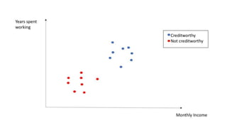
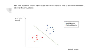
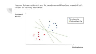
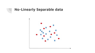
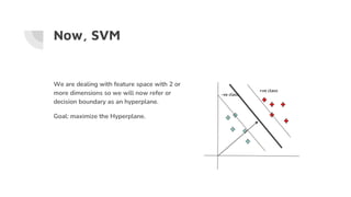
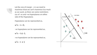
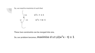
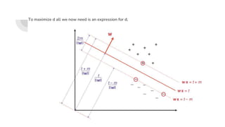
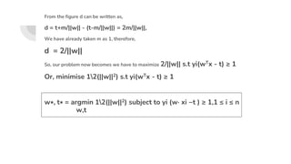
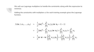
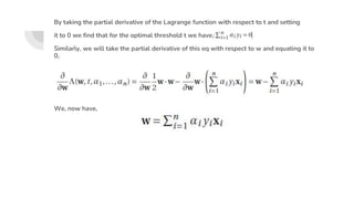
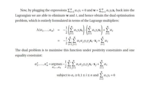
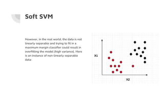
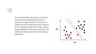
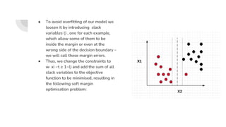
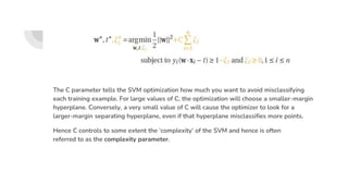
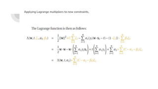
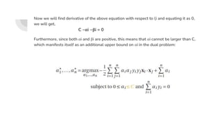
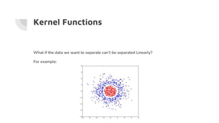
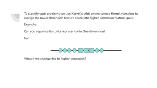
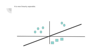
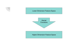
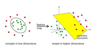
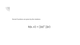
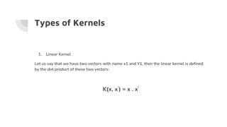
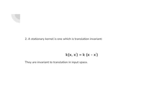
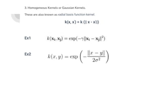
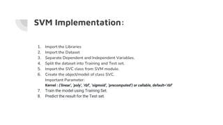
Support Vector Machines (SVM) find the optimal separating hyperplane that maximizes the margin between two classes of data points. The hyperplane is chosen such that it maximizes the distance from itself to the nearest data points of each class. When data is not linearly separable, the kernel trick can be used to project the data into a higher dimensional space where it may be linearly separable. Common kernel functions include linear, polynomial, radial basis function (RBF), and sigmoid kernels. Soft margin SVMs introduce slack variables to allow some misclassification and better handle non-separable data. The C parameter controls the tradeoff between margin maximization and misclassification.

1. Support Vector
Machine
And Kernel Functions
By Ms. Gunjan Rani
Assistant Professor
Acharya Narendra Dev College

2. Support Vector Machines (SVM), among classifiers, are probably
the most intuitive and elegant, especially for binary
classification tasks.

3. Linearly Separable data
Generally speaking, the idea of SVM is finding a frontier which separates observations into
classes.

5. Our SVM algorithm is then asked to find a boundary which is able to segregate those two
classes of clients, like so:

6. However, that was not the only way the two classes could have been separated. Let’s
consider the following alternatives:

7. Since we can separate observations in numerous ways, SVM is performed so that it can
finally find the boundary, called hyperplane, which best segregates the classes.
What does it mean “best segregating”?

8. The optimum hyperplane is the one which guarantees the largest “area of freedom” for
other future observations, an area where they can afford to deviate from their pattern
without undermining the model. The SVM, in particular, is looking for a boundary that is
maximally far away from any data point. This distance from that decision boundary to the
closest data points determines the margin of the classifier.
The best hyperplane is the one which maximizes the margin, under the constraint that each
data point must lie on the correct side of the margin.

10. Now a further concept needs to be
introduced. If you look at the graph:

11. Data points which are circled play a very important role in building the model. These data
points are called Support Vectors.

12. No-Linearly Separable data

13. There are two classes: squares and circles, however there is no way to trace a straight line
to segregate those classes. How shall we proceed?
The answer to this task is the reason why SVM became so popular, as there is a trick,
known as “Kernel Trick” from his inventor, which allows support vector machines to
effortlessly go from linear models to non-linear models by using only a slightly different
optimization problem from the one we have just seen.

14. What I want to do is providing an intuitive way to elaborate this task. Let’s see the idea
behind with this easy graph:

15. Again, you want to segregate squares from circles, and here a possible boundary might be
the one in green.
Now, the idea is the following: if we lift up the circles in a 3-dimensional plane, using a
given transformation function φ(x) we would be able to easily separate observations with
the support of a plan:

16. but how can we compute φ(x)?
Well, actually we are not asked to do so. Indeed, moving to a high-dimensional space is
the kernel functions’ job, which creates an implicit feature space.
Therefore, the transformation function φ(x) is not needed as we are provided with a list of
kernel functions, known also as “similarity functions” . The most popular is the Radial Basis
Function (RBF) kernel, or Gaussian kernel function, which looks like that:
With x and y being two vectors of features representing two different observations.

17. SVM Maths
Decision rule for any decision Boundary
during classification problems.
If we have a new data point say x(x1, x2),
we needt to determine which class it
belongs to.
We can clearly see, that x belongs to -ve
class but we need to have some decision
rule to make our machine understand which
class this x belongs to.
-ve class
+ve class

18. ● We take a vector perpendicular to
decision boundary such that we now
know direction of w but not its
magnitude.
● We now take a vector x and find its
projection on w vector which will be
nothing but the dot product of the
two vectors.
Vector w Vector x
projectio
n
t
-ve class
+ve class

19. Let’s say if the projection of x on w is greater than some constant, say t, then it belongs to
+ve class else it belongs to -ve class., or
-> w.x ≥ t, then y = +ve, or
-> w.x - t ≥ 0, then y = =ve
This is our decision rule which says.
y_pred = +ve
if wTx - t ≥ 0
else if wTx - t < 0
then y_pred = -ve

20. Now, SVM
We are dealing with feature space with 2 or
more dimensions so we will now refer or
decision boundary as an hyperplane.
Goal: maximize the Hyperplane.
-ve class
+ve class

21. Let the size of margin = d, we need to
maximise d but we can’t maximise d as much
as we want, as there are some restrictions
coz of -ve and +ve hyperplanes on either
side of the Hyperplane.
Hyperplane can be represented as,
wTx - t = 0,
-ve hyperplane can be represented as,
wTx - t ⪬ -1,
+ve hyperplane can be represented as,
wTx - t ≥ 1
-ve class
+ve class
d
+ve
-ve

22. So, we need to maximize d such that
+ve wTx - t ≥ 1
&
yi -ve wTx - t ⪬ -1
These two constraints can be merged into one,
So, our problem becomes, maximise d s.t yi(wTx - t) ≥ 1

23. To maximize d all we now need is an expression for d,

24. From the figure d can be written as,
d = t+m/||w|| - (t-m/||w||) = 2m/||w||,
We have already taken m as 1, therefore,
d = 2/||w||
So, our problem now becomes we have to maximize 2/||w|| s.t yi(wTx - t) ≥ 1
Or, minimise 12(||w||2) s.t yi(wTx - t) ≥ 1
w∗, t∗ = argmin 12(||w||2) subject to yi (w· xi −t ) ≥ 1,1 ≤ i ≤ n
w,t

25. We will use Lagrange multipliers to handle the constraints along with the expression to
minimize.
Adding the constraints with multipliers αi for each training example gives the Lagrange
function,

26. By taking the partial derivative of the Lagrange function with respect to t and setting
it to 0 we find that for the optimal threshold t we have,
Similarly, we will take the partial derivative of this eq with respect to w and equating it to
0,
We, now have,

28. Soft SVM
However, in the real world, the data is not
linearly separable and trying to fit in a
maximum margin classifier could result in
overfitting the model (high variance). Here
is an instance of non-linearly separable
data:

29. For the above data set which is non-linear
and not easily separable, trying to fit a
maximum margin classifier can result in a
model such as the following which looks to
be an overfitted model with a high variance.
It gets difficult for training to converge. The
model may fail to generalize for the larger
population.

30. ● To avoid overfitting of our model we
loosen it by introducing slack
variables ξi , one for each example,
which allow some of them to be
inside the margin or even at the
wrong side of the decision boundary –
we will call these margin errors.
● Thus, we change the constraints to
w· xi −t ≥ 1−ξi and add the sum of all
slack variables to the objective
function to be minimised, resulting in
the following soft margin
optimisation problem:

31. The C parameter tells the SVM optimization how much you want to avoid misclassifying
each training example. For large values of C, the optimization will choose a smaller-margin
hyperplane. Conversely, a very small value of C will cause the optimizer to look for a
larger-margin separating hyperplane, even if that hyperplane misclassifies more points.
Hence C controls to some extent the ‘complexity’ of the SVM and hence is often
referred to as the complexity parameter.

32. Applying Lagrange multipliers to new constraints,

33. Now we will find derivative of the above equation with respect to ξi and equating it as 0,
we will get,
C −αi −βi = 0
Furthermore, since both αi and βi are positive, this means that αi cannot be larger than C,
which manifests itself as an additional upper bound on αi in the dual problem:

34. Kernel Functions
What if the data we want to separate can’t be separated Linearly?
For example:

35. To classify such problems we use Kernel’s trick where we use Kernel functions to
change the lower dimension feature space into higher dimension feature space.
Example:
Can you separate this data represented in One dimension?
No!
What if we change this to higher dimension?

36. It is now linearly separable.

37. Lower Dimension Feature Space
Kernel
Functions
Higher DImension Feature Space

39. Kernel Functions are given by the relations:
k(x, x’) = Ⲫ(x)T Ⲫ(x’)

40. Types of Kernels
1. Linear Kernel
Let us say that we have two vectors with name x1 and Y1, then the linear kernel is defined
by the dot product of these two vectors:
K(x, x’) = x . x’

41. 2. A stationary kernel is one which is translation invariant:
k(x, x’) = k (x - x’)
They are invariant to translation in input space.

42. 3. Homogeneous Kernels or Gaussian Kernels.
These are also known as radial basis function kernel.
k(x, x’) = k (|| x - x'||)
Ex1
Ex2

43. SVM Implementation:
1. Import the Libraries
2. Import the Dataset
3. Separate Dependent and Independent Variables.
4. Split the dataset into Training and Test set.
5. Import the SVC class from SVM module.
6. Create the object/model of class SVC.
Important Parameter:
Kernel : {‘linear’, ‘poly’, ‘rbf’, ‘sigmoid’, ‘precomputed’} or callable, default=’rbf’
7. Train the model using Training Set.
8. Predict the result for the Test set.

44. SVM Numerical