This document summarizes the formulation of elasticity problems. It discusses the field equations, boundary conditions, and general solution strategies for elasticity problems. The fundamental problem can be formulated using either a displacement formulation or stress formulation. General solution strategies include direct, inverse, and semi-inverse methods. Mathematical methods for solving problems include analytical, approximate, and numerical techniques.

1. Lecture 5
Elasticity problem formulation
The Game
Print version Lecture on Theory of Elasticity and Plasticity of
Dr. D. Dinev, Department of Structural Mechanics, UACEG
5.1
Contents
1 Field equations review 1
2 Boundary conditions 2
3 Fundamental problem formulation 3
3.1 Displacement formulation . . . . . . . . . . . . . . . . . . . . . . . . . . . . . 3
3.2 Stress formulation . . . . . . . . . . . . . . . . . . . . . . . . . . . . . . . . . . 4
3.3 Principle of superposition . . . . . . . . . . . . . . . . . . . . . . . . . . . . . . 5
3.4 Saint-Venant’s principle . . . . . . . . . . . . . . . . . . . . . . . . . . . . . . . 5
4 General solution strategies 5
4.1 Direct method . . . . . . . . . . . . . . . . . . . . . . . . . . . . . . . . . . . . 5
4.2 Inverse method . . . . . . . . . . . . . . . . . . . . . . . . . . . . . . . . . . . 5
4.3 Semi-inverse method . . . . . . . . . . . . . . . . . . . . . . . . . . . . . . . . 6
4.4 Solution methods . . . . . . . . . . . . . . . . . . . . . . . . . . . . . . . . . . 6 5.2
1 Field equations review
Field equations review
Boundary Value Problem
• The field equations are differential and algebraic relations between strain, stresses and
displacements within the body
• We need of appropriate boundary conditions (BCs) to solve the elasticity problem. These
BCs specify the loading and supports that create stress, strain and displacement fields
• Field equations are same but the BCs are different
• Field Equations + Boundary Conditions = Boundary Value Problem
Note
• It is very important to imply proper BCs for a problem solution
5.3
Field equations review
Field Equations
• Strain-displacement relations- 6 pieces, 9 variables (6 strains+3 displacements)
εij =
1
2
(ui,j +uj,i) or ε =
1
2
∇u+(∇u)T
1

2. • Compatibility equations- 6 pieces (to check only)
εmn,ij +εij,mn = εim,jn +εjn,im or ∇×(∇×ε)T
= 0
• Equilibrium equations- 3 pieces, 6 variables (6 stresses)
σij,i + fj = 0 or ∇·σ +f = 0
5.4
Field equations review
Field Equations
• Constitutive equations- 6 pieces, 12 variables (6 stresses + 6 strains)
σij = 2µεij +λεkkδij or σ = 2µε +λtr(ε)I
• Recapitulation
– 15 unknowns (6 stresses + 6 strains + 3 displacements)
– 15 equations (6 → (ε −u) + 6 → (σ −ε) + 3 → (σ − f))
• Everything is OK. The elasticity problem can be solved!?!
5.5
2 Boundary conditions
Boundary conditions
Loading and supports
• The BCs specify how the body is loaded or supported
5.6
Boundary conditions
Loading and supports
• Stress BCs- specify the tractions at boundary
ti = njσji = ¯ti or t = σ ·n = ¯t
5.7
Boundary conditions
Loading and supports
• Displacement BCs- specify the displacements at boundary
ui = ¯ui or u = ¯u
5.8
2

3. Boundary conditions
Loading and supports
• Mixed BCs- specify the displacements or tractions at boundary
t = σ ·n = ¯t or u = ¯u
Note
• Don’t specify stress and displacements BCs at the same boundary simultaneously!
5.9
Boundary conditions
Example
u = ¯u
σ ·n = ¯t
• Using the above relations determine the displacement and stress BCs at the body’s bound-
aries
5.10
3 Fundamental problem formulation
3.1 Displacement formulation
Fundamental problem formulation
Displacement formulation
• We try to develop a reduced set of field equations with displacement unknowns
• Replacement of kinematic relations into Hooke’s law gives
σij = µ (ui,j +uj,i)+λuk,kδij
• And next into the equilibrium equations leads to
µui,j j +(µ +λ)uj,ji + fi = 0
5.11
Fundamental problem formulation
Displacement formulation
• In tensor form
µ∇2
u+(µ +λ)∇(∇·u)+f = 0
• The above expressions are known as Lamé-Navier equations
Note
• Method is useful with displacement BCs
• Avoid compatibility equations
• Mostly for 3D problems
5.12
3

4. Fundamental problem formulation
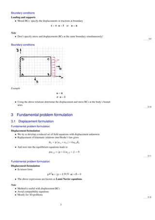
Displacement formulation
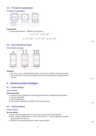
• Claude-Louis Navier (1785-1836)
5.13
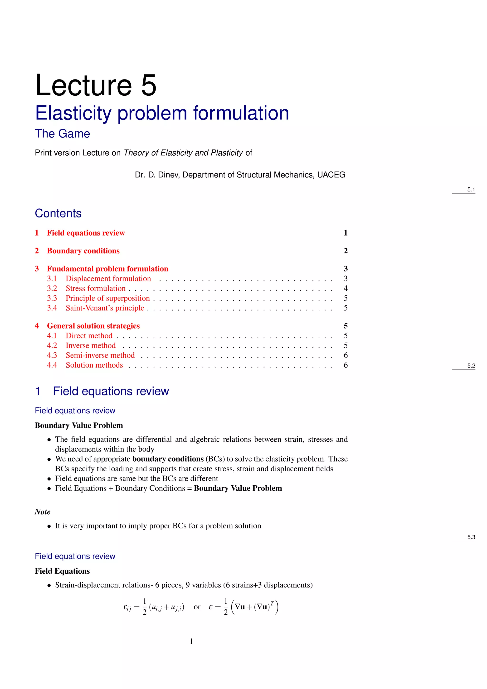
3.2 Stress formulation
Fundamental problem formulation
Stress formulation
• Stress-strain relations are replaced into compatibility equations
σij,kk +
1
1+ν
σkk,,ij = −
ν
1−ν
fk,kδij −(fj,i + fi,j)
• In tensor form
∇2
σ +
1
1+ν
∇[∇(tr∇)] = −
ν
1−ν
(∇·f)I− ∇f+(∇f)T
• The above expressions are known as Beltrami-Michell compatibility equations
Note
• Method is effective with stress BCs
• Need to work with compatibility eqns.
• Mostly for 2D problems
5.14
Fundamental problem formulation
Stress formulation
• Eugenio Beltrami (1835-1900)
5.15
4

5. 3.3 Principle of superposition
Principle of superposition
Superposition
• Linear field equations → Method of superposition
t = t(1)
+t(2)
, f = f(1)
+f(2)
σ = σ(1)
+σ(2)
, ε = ε(1)
+ε(2)
, u = u(1)
+u(2)
5.16
3.4 Saint-Venant’s principle
Saint-Venant’s principle
Definition
• The stress, strain, and displacement fields caused by two different statically equivalent
force distributions on parts of the body far away from the loading points are approximately
the same
5.17
4 General solution strategies
4.1 Direct method
Direct method
Direct integration
• Solution by direct integration of the field equations (stress or displacement formulation)
• Exactly satisfied BCs
• A lot of mathematics
• The method is applicable on problems with simple geometry
5.18
4.2 Inverse method
Inverse method
Reverse solution
• Select particular displacements or stresses that satisfy the basic field equations
• Seek a specific problem that fit to the solution field, i.e. find the appropriate problem
geometry, BCs and tractions
• Difficult to find practical problems to apply a given solution
5.19
5

6. 4.3 Semi-inverse method
Semi-inverse method
Direct + inverse method
• Part of the displacement or stress fields is specified
• The remaining portion - by direct integration of the basic field equations and BCs
• Start with approximate MoM solutions
• Enhancement by using the St-Venant’s principle
5.20
4.4 Solution methods
Solution methods
Mathematical methods for solutions
• Analytical solutions
– Power series method
– Fourier method
– Integral transform method etc.
• Approximate solution procedures
– Ritz method
– Bubnov-Galerkin method etc.
• Numerical solutions
– Finite difference method
– Finite element method
– Boundary element method
5.21
Solution methods
The End
• Any questions, opinions, discussions?
5.22
6