DIMENSIONAL ANALYSIS (Lecture notes 08)

CHAPTER 8
DIMENSIONAL ANALYSIS
8.1 INTRODUCTION
Dimensional analysis is one of the most important mathematical tools in the study of
fluid mechanics. It is a mathematical technique, which makes use of the study of dimensions
as an aid to the solution of many engineering problems. The main advantage of a dimensional
analysis of a problem is that it reduces the number of variables in the problem by combining
dimensional variables to form non-dimensional parameters.
By far the simplest and most desirable method in the analysis of any fluid problem is
that of direct mathematical solution. But, most problems in fluid mechanics such complex
phenomena that direct mathematical solution is limited to a few special cases. Especially for
turbulent flow, there are so many variables involved in the differential equation of fluid
motion that a direct mathematical solution is simply out of question. In these problems
dimensional analysis can be used in obtaining a functional relationship among the various
variables involved in terms of non-dimensional parameters.
Dimensional analysis has been found useful in both analytical and experimental work
in the study of fluid mechanics. Some of the uses are listed:
1) Checking the dimensional homogeneity of any equation of fluid motion.
2) Deriving fluid mechanics equations expressed in terms of non-dimensional
parameters to show the relative significance of each parameter.
3) Planning tests and presenting experimental results in a systematic manner.
4) Analyzing complex flow phenomena by use of scale models (model similitude).
8.2 DIMENSIONS AND DIMENSIONAL HOMOGENEITY
Scientific reasoning in fluid mechanics is based quantitatively on concepts of such
physical phenomena as length, time, velocity, acceleration, force, mass, momentum, energy,
viscosity, and many other arbitrarily chosen entities, to each of which a unit of measurement
has been assigned. For the purpose of obtaining a numerical solution, we adopt for
computation the quantities in SI or MKS units. In a more general sense, however, it is
desirable to adopt a consistent dimensional system composed of the smallest number of
dimensions in terms of which all the physical entities may be expressed. The fundamental
dimensions of mechanics are length [L], time [T], mass [M], and force [F], related by
Newton’s second law of motion, F = ma.
Prof. Dr. Atıl BULU130

Dimensionally, the law may also be written as,
[ ] ⎥
⎦
⎤
⎢
⎣
⎡
= 2
T
ML
F or 1
2
=⎥
⎦
⎤
⎢
⎣
⎡
ML
FT
(8.1)
Which indicates that when three of the dimensions are known, the fourth may be
expressed in the terms of the other three. Hence three independent dimensions are sufficient
for any physical phenomenon encountered in Newtonian mechanics. They are usually chosen
as either [MLT] (mass, length, time) or [FLT] (force, length, time). For example, the specific
mass (ρ) may be expressed either as [M/L3
]or as [FT2
/L4
], and a fluid pressure (p), which is
commonly expressed as force per unit area [F/L2
] may also be expressed as [ML/T2
] using the
(mass, length, time) system. A summary of some of the entities frequently used in fluid
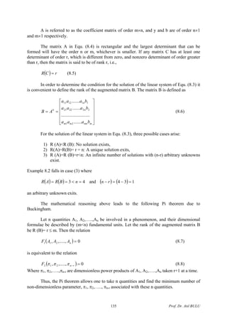
mechanics together with their dimensions in both systems is given in Table 8.1.
TABLE 8.1
ENTITIES COMMONLY USED IN FLUID MECHANICS
AND THEIR DIMENSIONS
Entity MLT System FLT System
Length (L) L L
Area (A) L2
L2
Volume (V) L3
L3
Time (t) T T
Velocity (v) LT-1
LT-1
Acceleration (a) LT-2
LT-2
Force (F) and weight (W) MLT-2
F
Specific weight (γ) ML-2
T-2
FL-3
Mass (m) M FL-1
T-2
Specific mass (ρ) ML-3
FL-4
T2
Pressure (p) and stress (τ) ML-1
T-2
FL-2
Energy (E) and work ML2
T-2
FL
Momentum (mv) MLT-1
FT
Power (P) ML2
T-3
FLT-1
Dynamic viscosity (μ) ML-1
T-1
FL-2
T
Kinematic viscosity (υ) L2
T-1
L2
T-1
With the selection of three independent dimensions –either [MLT] or [FLT]- it is
possible to express all physical entities of fluid mechanics. An equation which expresses the
physical phenomena of fluid motion must be both algebraically correct and dimensionally
homogenous. A dimensionally homogenous equation has the unique characteristic of being
independent of units chosen for measurement.
Equ. (8.1) demonstrates that a dimensionally homogenous equation may be
transformed to a non-dimensional form because of the mutual dependence of fundamental
dimensions. Although it is always possible to reduce dimensionally homogenous equation to a
non-dimensional form, the main difficulty in a complicated flow problem is in setting up the
correct equation of motion. Therefore, a special mathematical method called dimensional
analysis is required to determine the functional relationship among all the variables involved
in any complex phenomenon, in terms of non-dimensional parameters.

8.3 DIMENSIONAL ANALYSIS
The fact that a complete physical equation must be dimensionally homogenous and is,
therefore, reducible to a functional equation among non-dimensional parameters forms the
basis for the theory of dimensional analysis.
8.3.1 Statement of Assumptions
The procedure of dimensional analysis makes use of the following assumptions:
1) It is possible to select m independent fundamental units (in mechanics, m=3, i.e.,
length, time, mass or force).
2) There exist n quantities involved in a phenomenon whose dimensional formulae
may be expressed in terms of m fundamental units.
3) The dimensional quantity A0 can be related to the independent dimensional
quantities A1, A2, ......, An-1 by,
( ) 121
1211210 ......,.....,, −
−− == ny
n
yy
n AAKAAAAFA (8.2)
Where K is a non-dimensional constant, and y1, y2,.....,yn-1 are integer
components.
4) Equ. (8.2) is independent of the type of units chosen and is dimensionally
homogenous, i.e., the quantities occurring on both sides of the equation must
have the same dimension.
EXAMPLE 8.1: Consider the problem of a freely falling body near the surface of the
earth. If x, w, g, and t represent the distance measured from the initial height, the weight of
the body, the gravitational acceleration, and time, respectively, find a relation for x as a
function of w, g, and t.
SOLUTION: Using the fundamental units of force F, length L, and time T, we note
that the four physical quantities, A0=x, A1=w, A2=g, and A3=t, involve three fundamental
units; hence, m=3 and n=4 in assumptions (1) and (2). By assumption (3) we assume a
relation of the form:
( ) 321
,, yyy
tgKwtgwFx == (a)
Where K is an arbitrary non-dimensional constant.
Let [⋅] denote “dimensions of a quantity”. Then the relation above can be written
(using assumption (4)) as,
[ ] [ ] [ ] [ ] 321 yyy
tgwx =
or
( ) ( ) ( ) 3221321 22010 yyyyyyy
TLFTLTFTLF +−−
==

Equating like exponents, we obtain
2
1
1:
0:
yL
yF
=
=
3220: yyT +−= or 22 23 == yy
Therefore, Equ. (a) becomes
210
tgKwx =
or
2
Kgtx =
According to the elementary mechanics we have x=gt2
/2. The constant K in this case
is ½, which cannot be obtained from dimensional analysis.
EXAMPLE 8.2: Consider the problem of computing the drag force on a body moving
through a fluid. Let D, ρ, μ, l, and V be drag force, specific mass of the fluid, dynamic
viscosity of the fluid, body reference length, and body velocity, respectively.
SOLUTION: For this problem m=3, n=5, A0=D, A1=ρ, A2=μ, A3=l, and A4=V. Thus,
according to Equ (8.2), we have
( ) 4321
,,, yyyy
VlKVlFD μρμρ == (a)
or
[ ] [ ] [ ] [ ] [ ]
( ) ( ) ( ) ( )
421432121
4
3
21
4321
224001
1224001
yyyyyyyyy
yyyy
yyyy
TLFTLF
LTLTFLTFLTLF
VlD
−+++−−+
−−−
=
=
= μρ
Equating like exponents, we obtain
421
4321
21
20:
240:
1:
yyyT
yyyyL
yyF
−+=
++−−=
+=
In this case we have three equations and four unknowns. Hence, we can only solve for
three of the unknowns in terms of the fourth unknown (a one-parameter family of solutions
exists). For example, solving for y1, y3 and y4 in terms of y2, one obtains
24
23
21
2
2
1
yy
yy
yy
−=
−=
−=

The required solution is
2222 221 yyyy
VlKD −−−
= μρ
or
( ) 2
2
2
2
2
l
VVl
KD
y
⎟⎟
⎠
⎞
⎜⎜
⎝
⎛
⎟⎟
⎠
⎞
⎜⎜
⎝
⎛
=
−
ρ
μ
ρ
If the Reynolds number is denoted by Re=ρVl/μ, dynamic pressure by q=ρV2
/2, and
area by A=l2
, we have
( )
qACqA
K
D Dy
== 2
Re
2
where
( ) 2
Re
2
yD
K
C =
Theoretical considerations show that for laminar flow
328.12 =K and
2
1
2 =y
8.3.2 Buckingham-π (Pi) Theorem
It is seen from the preceding examples that m fundamental units and n physical
quantities lead to a system of m linear algebraic equations with n unknowns of the form
mnmnmm
nn
nn
byayaya
byayaya
byayaya
=+++
=+++
=+++
......
..................................................
......
.......
2211
22222121
11212111
(8.3)
or, in matrix form,
bAy = (8.4)
where
⎥
⎥
⎥
⎥
⎦
⎤
⎢
⎢
⎢
⎢
⎣
⎡
=
mnmm
n
n
aaa
aaa
aaa
A
......
......................
.......
.......
21
22212
11211
⎥
⎥
⎥
⎥
⎦
⎤
⎢
⎢
⎢
⎢
⎣
⎡
=
ny
y
y
y
.
2
1
and
⎥
⎥
⎥
⎥
⎦
⎤
⎢
⎢
⎢
⎢
⎣
⎡
=
nb
b
b
b
.
2
1

A is referred to as the coefficient matrix of order m×n, and y and b are of order n×1
and m×1 respectively.
The matrix A in Equ. (8.4) is rectangular and the largest determinant that can be
formed will have the order n or m, whichever is smaller. If any matrix C has at least one
determinant of order r, which is different from zero, and nonzero determinant of order greater
than r, then the matrix is said to be of rank r, i.e.,
( ) rCR = (8.5)
In order to determine the condition for the solution of the linear system of Equ. (8.3) it
is convenient to define the rank of the augmented matrix B. The matrix B is defined as
⎥
⎥
⎥
⎥
⎦
⎤
⎢
⎢
⎢
⎢
⎣
⎡
==
mmnmm
n
n
b
baaa
baaa
baaa
AB
.......
.........................
.......
.......
21
222221
111211
(8.6)
For the solution of the linear system in Equ. (8.3), three possible cases arise:
1) R (A)<R (B): No solution exists,
2) R(A)=R(B)= r = n: A unique solution exits,
3) R (A)=R (B)=r<n: An infinite number of solutions with (n-r) arbitrary unknowns
exist.
Example 8.2 falls in case (3) where
( ) ( ) 43 =<== nBRAR and ( ) ( ) 134 =−=− rn
an arbitrary unknown exits.
The mathematical reasoning above leads to the following Pi theorem due to
Buckingham.
Let n quantities A1, A2,…..,An be involved in a phenomenon, and their dimensional
formulae be described by (m<n) fundamental units. Let the rank of the augmented matrix B
be R (B)= r ≤ m. Then the relation
( 0,.....,, 211 =nAAAF ) (8.7)
is equivalent to the relation
( ) 0,.....,, 212 =−rnF πππ (8.8)
Where π1, π2,…..,πn-r are dimensionless power products of A1, A2,…..,An taken r+1 at a time.
Thus, the Pi theorem allows one to take n quantities and find the minimum number of
non-dimensionless parameter, π1, π2,….., πn-r associated with these n quantities.

8.3.2.1 Determination of Minimum Number of π Terms
In order to apply the Buckingham π Theorem to a given physical problem the
following procedure should be used:
Step 1. Given n quantities involving m fundamental units, set up the augmented
matrix B by constructing a table with the quantities on the horizontal axis and the
fundamental units on the vertical axis. Under each quantity list a column of numbers, which
represent the powers of each fundamental units that makes up its dimensions. For example,
ρ p d Q
F 1 1 0 1
L -4 -2 1 3
T 2 0 0 -1
Where ρ, p, d, and Q are the specific mass, pressure, diameter, and discharge,
respectively. The resulting array of numbers represents the augmented matrix B in
Buckingham’s π Theorem, i.e.,
⎥
⎥
⎥
⎦
⎤
⎢
⎢
⎢
⎣
⎡
−
−−=
1002
3124
0011
B
The matrix B is sometimes referred to as dimensional matrix.
Step 2. Having constructed matrix B, find its rank. From step1, since
01
002
024
011
≠=−−
and no larger nonzero determinant exists, then
( ) rBR == 3
Step3. Having determined the number of π dimensionless (n-r) terms, following rules
are used to combine the variables to form π terms.
a) From the independent variables select certain variables to use as repeating
variables, which will appear in more than π term. The repeating variables should
contain all the dimensions used in the problem and be quantities, which are likely
to have substantial effect on the dependent variable.
b) Combine the repeating variables with remaining variables to form the required
number of independent dimensionless π terms.
c) The dependent variable should appear in one group only.
d) A variable that is expected to have a minor influence should appear in one group
only.

Define π1 as a power product of r of the n quantities raised to arbitrary integer
exponents and any one of the excluded (n-r) quantities, i.e.,
1211
11211
..... += r
y
r
yy
AAAA r
π
Step 4. Define π2, π3,....., πn-r as power products of the same r quantities used in step 3
raised to arbitrary integer exponents but a different excluded quantity for each π term, i.e.,
n
y
r
yy
rn
r
y
r
yy
r
y
r
yy
AAAA
AAAA
AAAA
rrnrnrn
r
r
,2,1,
33231
22221
.....
........................................
.............
.............
21
3213
2212
−−−
=
=
=
−
+
+
π
π
π
Step 5. Carry out dimensional analysis on each π term to evaluate the exponents.
EXAMPLE 8.3: Rework Example 8.1 using the π theorem.
SOLUTION:
Step 1. With F, L, and T as the fundamental units, the dimensional matrix of the
quantities w, g, t and x is,
W g t x
F 1 0 0 0
L 0 1 0 1
T 0 -2 1 0
Where
⎥
⎥
⎥
⎦
⎤
⎢
⎢
⎢
⎣
⎡
−
=
0120
1010
0001
B
Step 2. Since
02
020
110
001
≠=
−
( ) rBR == 3
Step 3. Arbitrarily select x, w, and g as the r = m= 3 base quantities. The number n-r
of independent dimensional products that can be formed by the four quantities is therefore 1,
i.e.,
tgwx yyy 131211
1 =π

Step 4. Dimensional analysis gives,
[ ] [ ] [ ] [ ] [ ]tgwx
yyy 131211
1 =π
or
( ) ( ) ( ) ( )TLTFLTLF
yyy 131211 2000 −
=
Which results in
2
1
11 −=y , 012 =y , and
2
1
13 =y
Hence,
x
gt2
1 =π
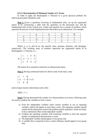
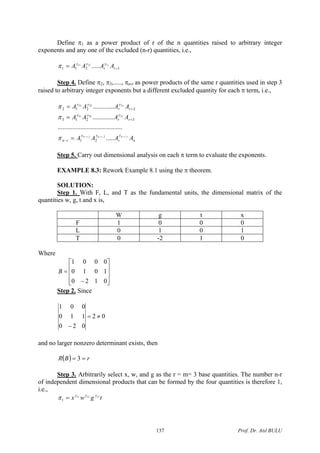
EXAMPLE 8.4: Rework Example 8.2 using the π theorem.
SOLUTION:
Step 1. With F, L and T as the fundamental units, the dimensional matrix of the
quantities D, ρ, μ, l, and V is.
D ρ μ l V
F 1 1 1 0 0
L 0 -4 -2 1 1
T 0 2 1 0 -1
Where
⎥
⎥
⎥
⎦
⎤
⎢
⎢
⎢
⎣
⎡
−
−−=
10120
11240
00111
B
Step2. Since
01
101
112
001
≠=
−
−
( ) rBR == 3

Step 3. Select l, V, and ρ as the r=3 base quantities. By the π-Theorem (n-r),(5-3)=2 π
terms exist.
μρπ
ρπ
232221
131211
2
1
yyy
yyy
Vl
DVl
=
=
Step 4. Dimensional analysis gives
y11=-2, y12=-2, y13= -1
y21=-1, y22=-1, y23=-1
Hence,
Vl
lV
D
ρ
μ
π
ρ
π
=
=
2
221
8.4 THE USE OF DIMENSIONLESS π-TERMS IN EXPERIMENTAL
INVESTIGATIONS
Dimensional analysis can be of assistance in experimental investigation by reducing
the number of variables in the problem. The result of the analysis is to replace an unknown
relation between n variables by a relationship between a smaller numbers, n-r, of
dimensionless π-terms. Any reduction in the number of variables greatly reduces the labor of
experimental investigation. For instance, a function of one variable can be plotted as a single
curve constructed from a relatively small number of experimental observations, or the results
can be represented as a single table, which might require just one page.
A function of two variables will require a chart consisting of a family of curves, one
for each value of the second variable, or, alternatively the information can be presented in the
form of a book of tables. A function of three variables will require a set of charts or a shelf-
full of books of tables.
As the number of variables increases, the number of observations to be taken grows so
rapidly that the situation soon becomes impossible. Any reduction in the number of variables
is extremely important.
Considering, as an example, the resistance to flow through pipes, the shear stress or
resistance R per unit area at the pipe wall when fluid of specific mass ρ and dynamic viscosity
μ flows in a smooth pipe can be assumed to depend on the velocity of flow V and the pipe
diameter D. Selecting a number of different fluids, we could obtain a set of curves relating
frictional resistance (measured as R/ρV2
) to velocity, as shown in Fig. 8.1.

0.015
Water,d=50.80mmWater,d=25.40mmWater,d=62.70mm
Air,d=25.40mm
Air,d=12.70mm
Air,d=6.35mm
0.010
0.005
0
0.01 0.1 1 10 100
v ( ms )-1
R/pv2 All measurements at 15.5°C
Fig. 8.1
Such a set of curves would be of limited value both for use and for obtaining a proper
understanding of the problem. However, it can be shown by dimensional analysis that the
relationship can be reduced to the form
( )Re2
φ
μ
ρ
φ
ρ
=⎟⎟
⎠
⎞
⎜⎜
⎝
⎛
=
VD
V
R
or, using the Darcy resistance coefficient 2
2 VRf ρ= ,
( )Reφ
μ
ρ
φ =⎟⎟
⎠
⎞
⎜⎜
⎝
⎛
=
VD
f
4
-3
10
10 2
2
10
-2
7
2
2 4 7 10
3
10
4
7
-1
5
10
Reynolds number , Re
2 4 7 10
4
42 7 102 4 7
6
Frictioncoefficient,f
Fig. 8.2

If the experimental points in Fig. 8.1 are used to construct a new graph of Log (f)
against Log (Re) the separate sets of experimental data combine to give a single curve as
shown in Fig. 8.2. For low values of Reynolds number, when flow is laminar, the slope of this
graph is (-1) and f = 16/Re, while for turbulent flow at higher values of Reynolds number,
f = 0.08(Re)-1/4
.

DIMENSIONAL ANALYSIS (Lecture notes 08)

Recommended

Recommended

More Related Content

What's hot

What's hot (20)

Viewers also liked

Viewers also liked (20)

Similar to DIMENSIONAL ANALYSIS (Lecture notes 08)

Similar to DIMENSIONAL ANALYSIS (Lecture notes 08) (20)

More from Shekh Muhsen Uddin Ahmed

More from Shekh Muhsen Uddin Ahmed (20)

Recently uploaded

Recently uploaded (20)

DIMENSIONAL ANALYSIS (Lecture notes 08)