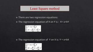
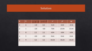
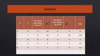
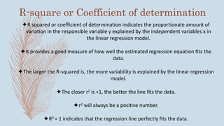
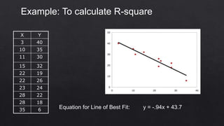
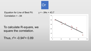
By
Shivangi Sarabhai, Simran Sakshi
& Sonam Kharwar
BBM
DEI
Contents
INTRODUCTION
o The dictionary meaning of the term “Regression” is the act of
returning or going back.
o The term regression was first used by sir “Francis Galton” in
1877 while studying the relationship between the height of
fathers and sons.
o This term introduced by him in the paper “Regression towards
mediocrity in hereditary stature”.
o “Regression is the measure of the average relationship
between two or more variables in terms of the original units of
the data.”
- Blair
“The term regression analysis refers to the methods by which
estimates are made of the variables from a knowledge of the
values of one or more other variables and to the measurement
of the errors involved in the estimation.”
- Morris Hamburg
Definition of Regression
Difference between Correlation and
Regression
S. NO.
Correlation Regression
1. Correlation coefficient is a
measure of degree of co-
variability or association
between X and Y.
The objective of regression
analyses is to the study of
nature of relationship
between the variables so
that we may be able to
predict the values of one on
the basis of another.
S. NO Correlation Regression
2. It is merely a tool of ascertaining
the degree of relationship
between two variable and,
therefore, we cannot say that
one variable is the cause and
the other is effect. The variables
may be affected by some
unknown common factor.
In regression analysis one variable is
taken as dependent while the other as
independent-thus making it possible to
study the cause and effect relationship.
3. Correlation coefficient is
independent of change of scale
and origin.
Regression coefficient is independent
of change of origin but not of scale.
S.
NO
Correlation Regression
4. In this 𝑟𝑥𝑦 is a measure of direction
and degree of linear relationship
between two variable X and Y. 𝑟𝑦𝑥
and 𝑟𝑥𝑦 are symmetric, it is
immaterial which of X and Y is
dependent variable and which is
independent variable.
In regression analyses the regression
coefficients 𝑏 𝑥𝑦 and 𝑏 𝑦𝑥 are not
symmetric, and hence it definitely
makes a difference as to which
variable is dependent and which is
independent.
Types of Regression
Linear Regression Logical Regression
Polynomial
Regression
Stepwise
Regression
Ridge Regression Lasso Regression
Linear Regression
Logistic Regression
Polynomial regression
Y= b0 + b1x + Ԑ
E(Y) = b0 + b1x
Ŷ = b0 + b1x
SIMPLE LINEAR REGRESSION MODEL
SIMPLE LINEAR REGRESSION EQUATION
ESTIMATED SIMPLE LINEAR REGRESSION EQUATION
REGRESSION
GRAPHICALLY FREE HAND CURVE
LEAST SQUARES
ALGEBRAICALLY
LEAST SQUARES
DEVIATION
METHOD FROM
ARITHMETIC
MEAN
DEVIATION
METHOD FROM
ASSUMED MEAN
Least Square Method
 A procedure for using sample data to find the estimated regression equation.
 It uses the sample data method to provide the values of b0 and b1 that minimize
the sum of the squares of the deviations between the observed values of the
dependent variable Y and the estimated values of the dependent variable Ŷ.
 The criterion for the least squares method is given as: min ∑(Yi – Ŷi)2
 The error on either side of the regression line has to be minimized.
 
 


2
YbYaXY
YbnaX
 
 


2
XbXaXY
XbnaY
X Y XY X2 Y2
3 6 18 9 36
2 1 2 4 1
7 8 56 49 64
4 5 20 16 25
8 9 72 64 81
 
 


2
YbYaXY
YbnaX
 
 


2
XbXaXY
XbnaY
X=0.49+0.74Y
)()( YYbXX xy 
)()( XXbYY yx 

 2
y
xy
bxy

 2
x
xy
byx
xyb yxb
X Y x2 y2 xy
3 6 -1.8 0.2 3.24 0.04 -0.36
2 1 -2.8 -4.8 7.84 23.04 13.44
7 8 2.2 2.2 4.84 4.84 4.84
4 5 -0.8 -0.8 0.64 0.64 0.64
8 9 3.2 3.2 10.24 10.24 10.24
XXx  YYy 
)()( YYbXX xy 
 
 
49.074.0
8.574.08.4
8.5
8.38
8.28
8.4
2






YX
YX
YX
y
xy
bxy
)()( XXbYY yx 
 
66.007.1
)8.4(07.18.5
8.4
8.26
8.28
8.5
2






XY
XY
XY
x
xy
byx
)()( YYbXX xy 
)()( XXbYY yx 
xyb yxb
  
  


 22
yy
yxyx
xy
ddN
ddddN
b
  
  


 22
xx
yxyx
yx
ddN
ddddN
b
X Y
Dev. From
assu. Mean
7 (dx)=X-7
Dev. From
assu. Mean 6
(dy)=Y-6 dxdy
3 6 -4 16 0 0 0
2 1 -5 25 -5 25 +25
7 8 0 0 2 4 0
4 5 -3 9 -1 1 +3
8 9 1 1 3 9 +3
2
xd 2
yd
  
  


 22
yy
yxyx
xy
ddN
ddddN
b
74.0
194
144
1195
11155
)1()39(5
)1)(11()31(5
2








xy
xy
xy
xy
b
b
b
b
49.074.0
)8.5(74.0)8.4(
)()(



YX
YX
YYbXX xy
  
  


 22
xx
yxyx
yx
ddN
ddddN
b
07.1
134
144
121255
11155
)11()51(5
)1)(11()31(5
2








yx
yx
yx
yx
b
b
b
b
)()( XXbYY yx 
66.007.1
)8.4(07.1)8.5(


XY
XY
R-square or Coefficient of determination
R squared or coefficient of determination indicates the proportionate amount of
variation in the responsible variable y explained by the independent variables x in
the linear regression model.
It provides a good measure of how well the estimated regression equation fits the
data.
The larger the R-squared is, the more variability is explained by the linear regression
model.
The closer r2 is +1, the better the line fits the data.
r2 will always be a positive number.
R2 = 1 indicates that the regression line perfectly fits the data.
X Y
3 40
10 35
11 30
15 32
22 19
22 26
23 24
28 22
28 18
35 6 Equation for Line of Best Fit: y = -.94x + 43.7
Example: To calculate R-square
X Y
Predicted Y
Value
Error
(predicted
value-y)
Error
Squared
Distance
between Y values
and their mean
Mean
distances
squared
3 40 40.88 .88 .77 14.8 219.04
10 35 34.30 -.70 .49 9.8 96.04
11 30 33.36 3.36 11.29 4.8 23.04
15 32 29.60 -2.40 5.76 6.8 46.24
22 19 23.02 4.02 16.16 -6.2 38.44
22 26 23.02 -2.98 8.88 .8 .64
23 24 22.08 -1.92 3.69 -1.2 1.44
28 22 17.38 -4.62 21.34 -3.2 10.24
28 18 17.38 -.62 .38 -7.2 51.84
35 6 10.80 4.8 23.04 -19.2 368.65
Mean: 25.2 Sum: 91.81 Sum: 855.60
Equation for Line of Best Fit: y = -.94x + 43.7
1-
Sum of squared distances between the
actual and predicted Y values
Sum of squared distances between the
actual Y values and their mean
1-
91.81
855.60
= 1- 0.11
= 0.89
R2 =
Or
Correlation = -.94
To calculate R-square, we
square the correlation.
Thus, r2= -0.942= 0.89
Equation for Line of Best Fit: y = -.94x + 43.7
 Adjusted R-square is a modification of R-square that adjusts
for the number of terms in a model.
 R-square always increases when a new term is added to a
model, but adjusted R-square increases only if the new term
improves the model more than would be expected by chance.
 This makes Adjusted R-square more useful for comparing
models with a different number of predictors.
 R-squared increases if we increase the number of
variables in the regression model.
R squared, a property of the fitted model, is a structure with two fields:
•Ordinary — Ordinary (unadjusted) R-squared
•Adjusted — R-squared adjusted for the number of coefficients
Uses of Regression Analysis
Helps in establishing a functional relationship between two or more
variables
As most of the problems of economic analysis is based on cause and
effect relationships, regression analysis is a highly valuable tool in
economics and business research
It predicts the values of dependent variables from the values of
independent variables
We can calculate the coefficient of correlation and coefficient of
determination with the help of regression coefficients
APPLICATIONS
 Regression.xlsx
o In making estimates from a regression equation, it
is important to remember that the assumption is
being made that relationship has not changed since
the regression equation was computed.
Another point worth remembering is that
relationship shown by the scatter diagram, may not
be the same if the equation is extended beyond the
values used in computing the equation.
Limitations of Regression
o for example
there may be a close linear relationship between
the yield of a crop and the amount of fertilizer
applied, with the yield increasing as the amount
of fertilizer is increased. It would not be logical,
however, to extend this equation beyond the
limits of experiment for it is quite likely that if the
amount of fertilizer were increase indefinitely, the
yield would eventually decline as too much
fertilizer was applied.
References
 http://www.hedgefund-index.com/d_rsquared.asp
 http://www.ats.ucla.edu/stat/stata/faq/mi_r_squared.htm
 http://in.mathworks.com/help/stats/coefficient-of-determination-r-squared.html?requestedDomain=www.mathworks.com
 http://www.graphpad.com/guides/prism/6/curve-fitting/index.htm?r2_ameasureofgoodness_of_fitoflinearregression.htm
 http://blog.minitab.com/blog/statistics-and-quality-data-analysis/r-squared-sometimes-a-square-is-just-a-square
 http://blog.minitab.com/blog/adventures-in-statistics/regression-analysis-tutorial-and-examples
Regression

Regression

  • 1.
    By Shivangi Sarabhai, SimranSakshi & Sonam Kharwar BBM DEI
  • 2.
  • 3.
    INTRODUCTION o The dictionarymeaning of the term “Regression” is the act of returning or going back. o The term regression was first used by sir “Francis Galton” in 1877 while studying the relationship between the height of fathers and sons. o This term introduced by him in the paper “Regression towards mediocrity in hereditary stature”.
  • 4.
    o “Regression isthe measure of the average relationship between two or more variables in terms of the original units of the data.” - Blair “The term regression analysis refers to the methods by which estimates are made of the variables from a knowledge of the values of one or more other variables and to the measurement of the errors involved in the estimation.” - Morris Hamburg Definition of Regression
  • 5.
    Difference between Correlationand Regression S. NO. Correlation Regression 1. Correlation coefficient is a measure of degree of co- variability or association between X and Y. The objective of regression analyses is to the study of nature of relationship between the variables so that we may be able to predict the values of one on the basis of another.
  • 6.
    S. NO CorrelationRegression 2. It is merely a tool of ascertaining the degree of relationship between two variable and, therefore, we cannot say that one variable is the cause and the other is effect. The variables may be affected by some unknown common factor. In regression analysis one variable is taken as dependent while the other as independent-thus making it possible to study the cause and effect relationship. 3. Correlation coefficient is independent of change of scale and origin. Regression coefficient is independent of change of origin but not of scale.
  • 7.
    S. NO Correlation Regression 4. Inthis 𝑟𝑥𝑦 is a measure of direction and degree of linear relationship between two variable X and Y. 𝑟𝑦𝑥 and 𝑟𝑥𝑦 are symmetric, it is immaterial which of X and Y is dependent variable and which is independent variable. In regression analyses the regression coefficients 𝑏 𝑥𝑦 and 𝑏 𝑦𝑥 are not symmetric, and hence it definitely makes a difference as to which variable is dependent and which is independent.
  • 8.
    Types of Regression LinearRegression Logical Regression Polynomial Regression Stepwise Regression Ridge Regression Lasso Regression
  • 9.
  • 10.
  • 11.
  • 12.
    Y= b0 +b1x + Ԑ E(Y) = b0 + b1x Ŷ = b0 + b1x SIMPLE LINEAR REGRESSION MODEL SIMPLE LINEAR REGRESSION EQUATION ESTIMATED SIMPLE LINEAR REGRESSION EQUATION
  • 13.
    REGRESSION GRAPHICALLY FREE HANDCURVE LEAST SQUARES ALGEBRAICALLY LEAST SQUARES DEVIATION METHOD FROM ARITHMETIC MEAN DEVIATION METHOD FROM ASSUMED MEAN
  • 14.
    Least Square Method A procedure for using sample data to find the estimated regression equation.  It uses the sample data method to provide the values of b0 and b1 that minimize the sum of the squares of the deviations between the observed values of the dependent variable Y and the estimated values of the dependent variable Ŷ.  The criterion for the least squares method is given as: min ∑(Yi – Ŷi)2  The error on either side of the regression line has to be minimized.
  • 15.
          2 YbYaXY YbnaX      2 XbXaXY XbnaY
  • 17.
    X Y XYX2 Y2 3 6 18 9 36 2 1 2 4 1 7 8 56 49 64 4 5 20 16 25 8 9 72 64 81
  • 18.
  • 19.
  • 21.
    )()( YYbXX xy )()( XXbYY yx    2 y xy bxy   2 x xy byx xyb yxb
  • 23.
    X Y x2y2 xy 3 6 -1.8 0.2 3.24 0.04 -0.36 2 1 -2.8 -4.8 7.84 23.04 13.44 7 8 2.2 2.2 4.84 4.84 4.84 4 5 -0.8 -0.8 0.64 0.64 0.64 8 9 3.2 3.2 10.24 10.24 10.24 XXx  YYy 
  • 24.
    )()( YYbXX xy     49.074.0 8.574.08.4 8.5 8.38 8.28 8.4 2       YX YX YX y xy bxy
  • 25.
    )()( XXbYY yx   66.007.1 )8.4(07.18.5 8.4 8.26 8.28 8.5 2       XY XY XY x xy byx
  • 27.
    )()( YYbXX xy )()( XXbYY yx  xyb yxb          22 yy yxyx xy ddN ddddN b          22 xx yxyx yx ddN ddddN b
  • 29.
    X Y Dev. From assu.Mean 7 (dx)=X-7 Dev. From assu. Mean 6 (dy)=Y-6 dxdy 3 6 -4 16 0 0 0 2 1 -5 25 -5 25 +25 7 8 0 0 2 4 0 4 5 -3 9 -1 1 +3 8 9 1 1 3 9 +3 2 xd 2 yd
  • 30.
            22 yy yxyx xy ddN ddddN b 74.0 194 144 1195 11155 )1()39(5 )1)(11()31(5 2         xy xy xy xy b b b b
  • 31.
  • 32.
            22 xx yxyx yx ddN ddddN b 07.1 134 144 121255 11155 )11()51(5 )1)(11()31(5 2         yx yx yx yx b b b b
  • 33.
    )()( XXbYY yx 66.007.1 )8.4(07.1)8.5(   XY XY
  • 34.
    R-square or Coefficientof determination R squared or coefficient of determination indicates the proportionate amount of variation in the responsible variable y explained by the independent variables x in the linear regression model. It provides a good measure of how well the estimated regression equation fits the data. The larger the R-squared is, the more variability is explained by the linear regression model. The closer r2 is +1, the better the line fits the data. r2 will always be a positive number. R2 = 1 indicates that the regression line perfectly fits the data.
  • 35.
    X Y 3 40 1035 11 30 15 32 22 19 22 26 23 24 28 22 28 18 35 6 Equation for Line of Best Fit: y = -.94x + 43.7 Example: To calculate R-square
  • 36.
    X Y Predicted Y Value Error (predicted value-y) Error Squared Distance betweenY values and their mean Mean distances squared 3 40 40.88 .88 .77 14.8 219.04 10 35 34.30 -.70 .49 9.8 96.04 11 30 33.36 3.36 11.29 4.8 23.04 15 32 29.60 -2.40 5.76 6.8 46.24 22 19 23.02 4.02 16.16 -6.2 38.44 22 26 23.02 -2.98 8.88 .8 .64 23 24 22.08 -1.92 3.69 -1.2 1.44 28 22 17.38 -4.62 21.34 -3.2 10.24 28 18 17.38 -.62 .38 -7.2 51.84 35 6 10.80 4.8 23.04 -19.2 368.65 Mean: 25.2 Sum: 91.81 Sum: 855.60 Equation for Line of Best Fit: y = -.94x + 43.7
  • 37.
    1- Sum of squareddistances between the actual and predicted Y values Sum of squared distances between the actual Y values and their mean 1- 91.81 855.60 = 1- 0.11 = 0.89 R2 =
  • 38.
    Or Correlation = -.94 Tocalculate R-square, we square the correlation. Thus, r2= -0.942= 0.89 Equation for Line of Best Fit: y = -.94x + 43.7
  • 39.
     Adjusted R-squareis a modification of R-square that adjusts for the number of terms in a model.  R-square always increases when a new term is added to a model, but adjusted R-square increases only if the new term improves the model more than would be expected by chance.  This makes Adjusted R-square more useful for comparing models with a different number of predictors.  R-squared increases if we increase the number of variables in the regression model. R squared, a property of the fitted model, is a structure with two fields: •Ordinary — Ordinary (unadjusted) R-squared •Adjusted — R-squared adjusted for the number of coefficients
  • 40.
    Uses of RegressionAnalysis Helps in establishing a functional relationship between two or more variables As most of the problems of economic analysis is based on cause and effect relationships, regression analysis is a highly valuable tool in economics and business research It predicts the values of dependent variables from the values of independent variables We can calculate the coefficient of correlation and coefficient of determination with the help of regression coefficients
  • 41.
  • 42.
    o In makingestimates from a regression equation, it is important to remember that the assumption is being made that relationship has not changed since the regression equation was computed. Another point worth remembering is that relationship shown by the scatter diagram, may not be the same if the equation is extended beyond the values used in computing the equation. Limitations of Regression
  • 43.
    o for example theremay be a close linear relationship between the yield of a crop and the amount of fertilizer applied, with the yield increasing as the amount of fertilizer is increased. It would not be logical, however, to extend this equation beyond the limits of experiment for it is quite likely that if the amount of fertilizer were increase indefinitely, the yield would eventually decline as too much fertilizer was applied.
  • 44.
    References  http://www.hedgefund-index.com/d_rsquared.asp  http://www.ats.ucla.edu/stat/stata/faq/mi_r_squared.htm http://in.mathworks.com/help/stats/coefficient-of-determination-r-squared.html?requestedDomain=www.mathworks.com  http://www.graphpad.com/guides/prism/6/curve-fitting/index.htm?r2_ameasureofgoodness_of_fitoflinearregression.htm  http://blog.minitab.com/blog/statistics-and-quality-data-analysis/r-squared-sometimes-a-square-is-just-a-square  http://blog.minitab.com/blog/adventures-in-statistics/regression-analysis-tutorial-and-examples