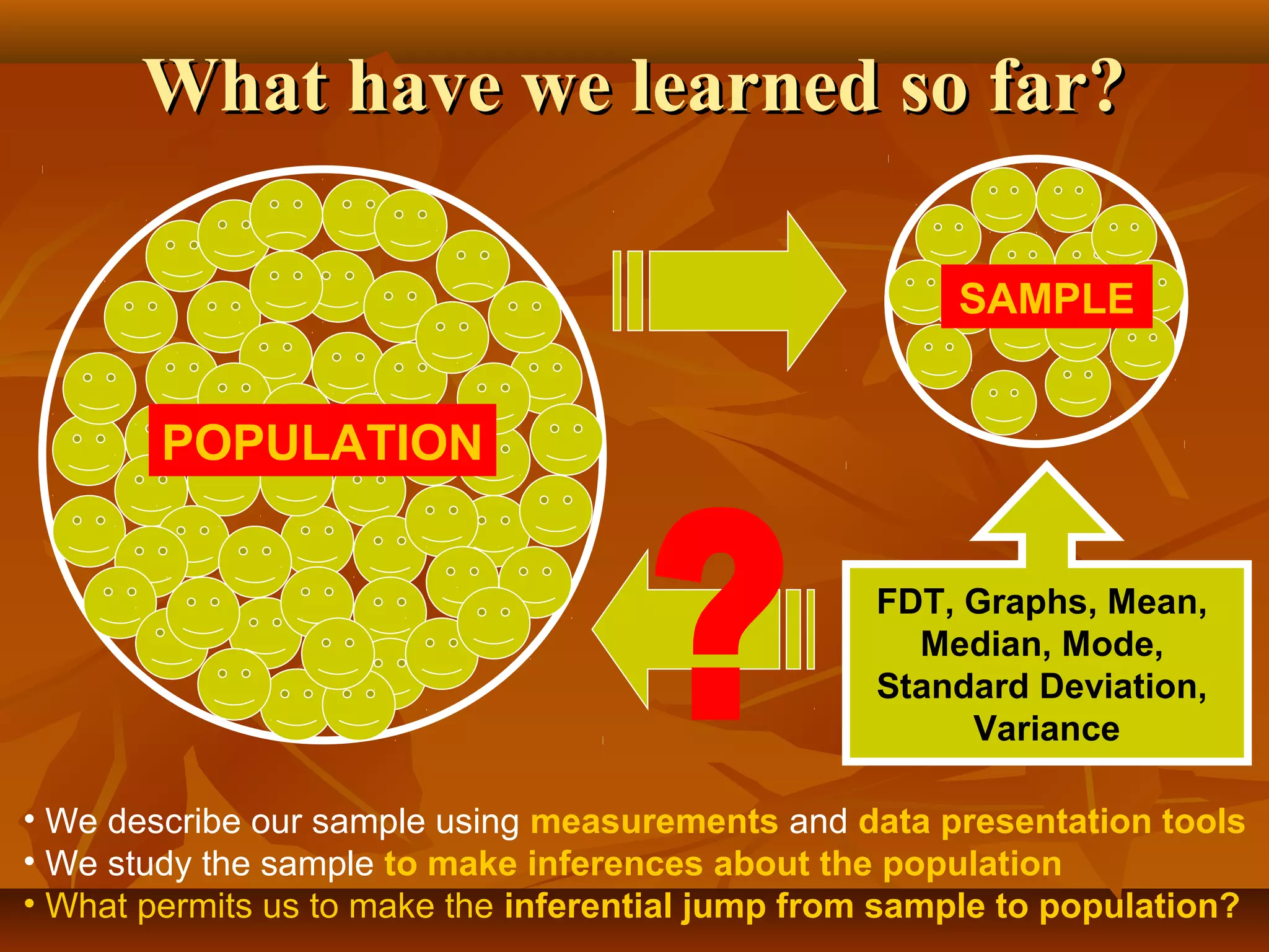
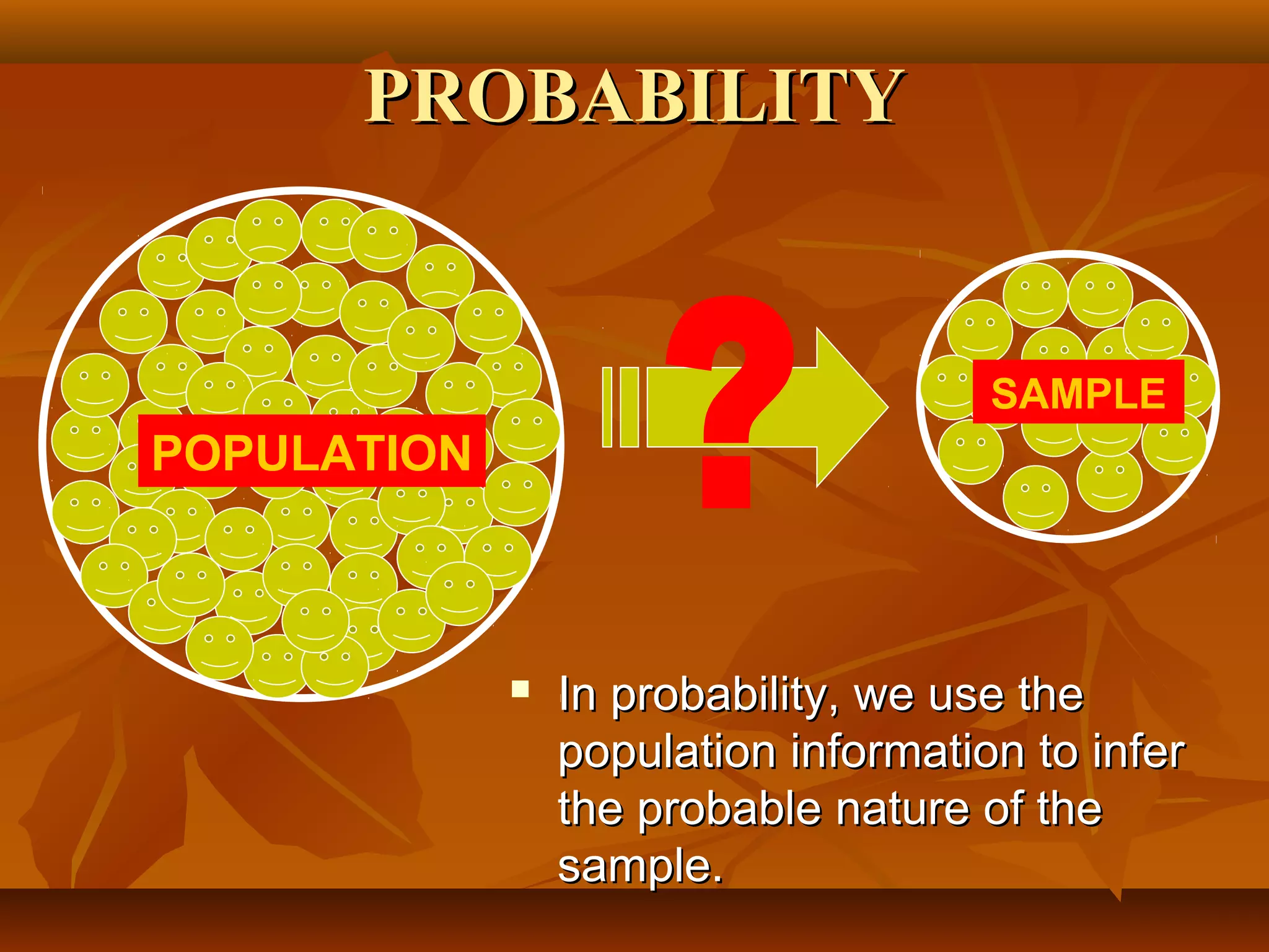
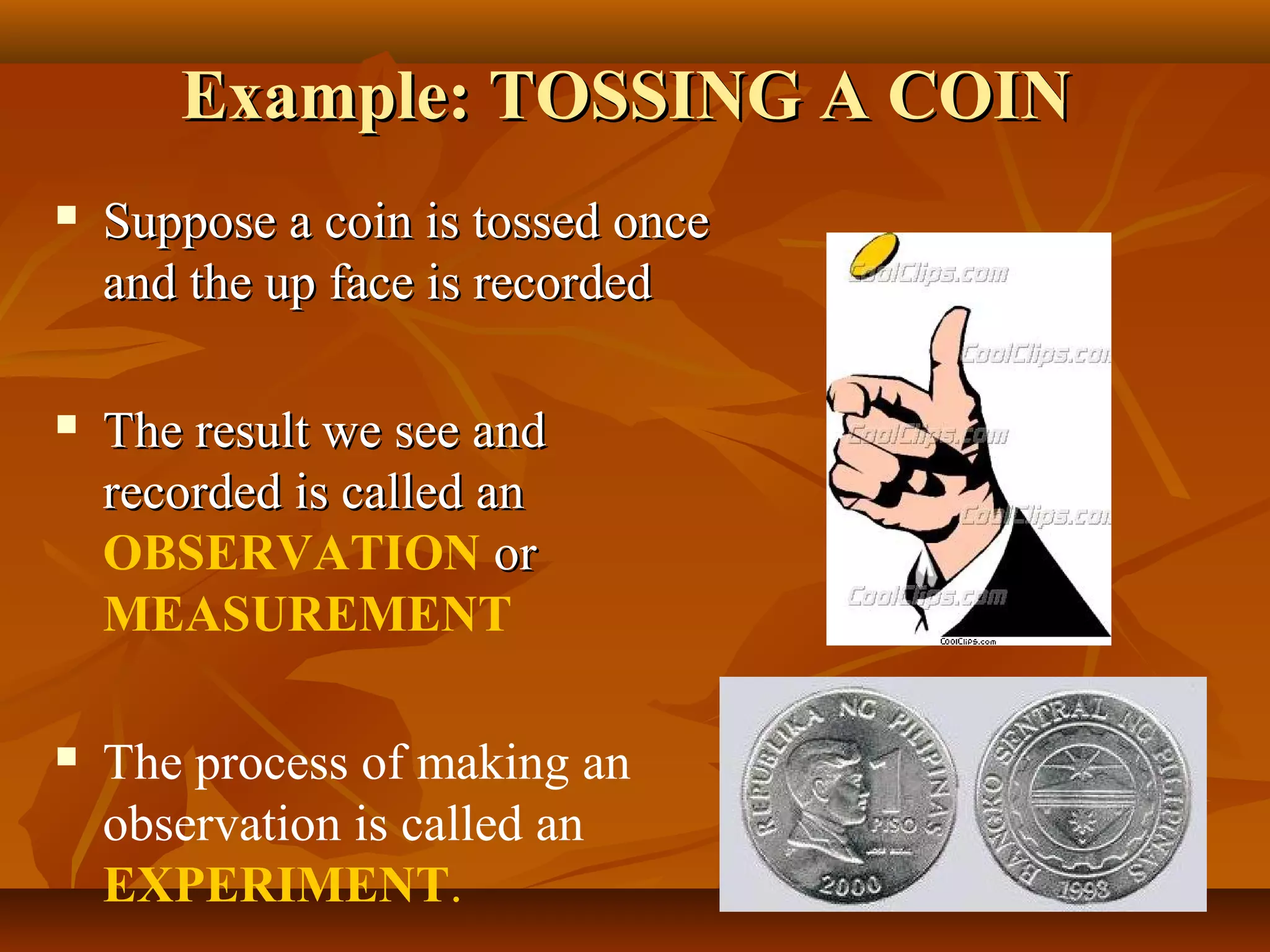
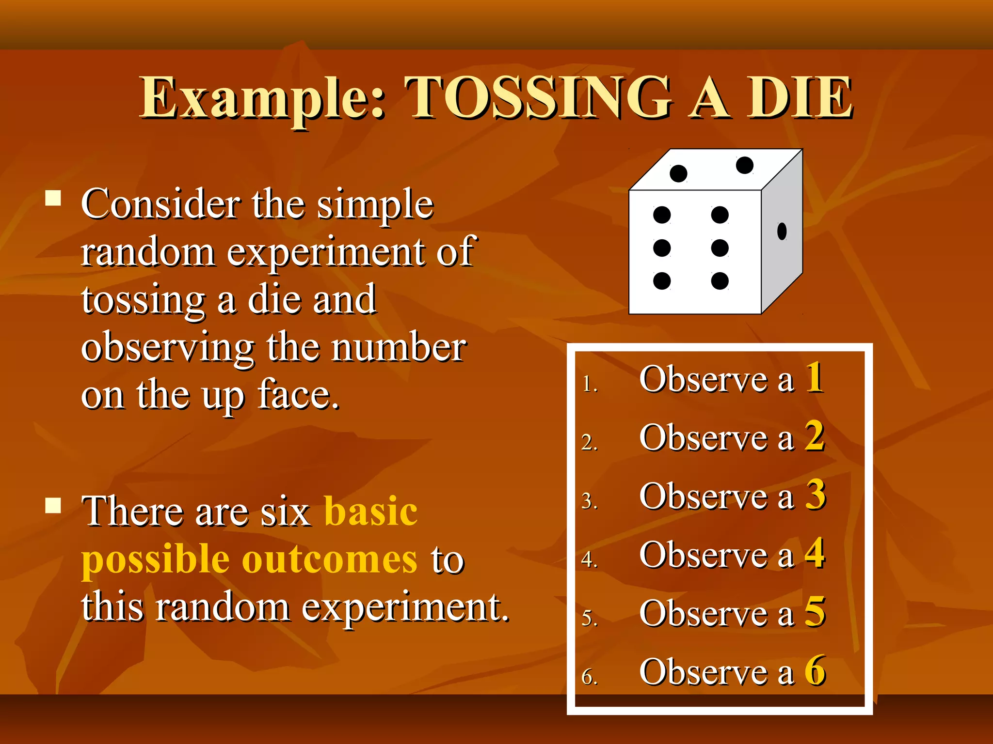
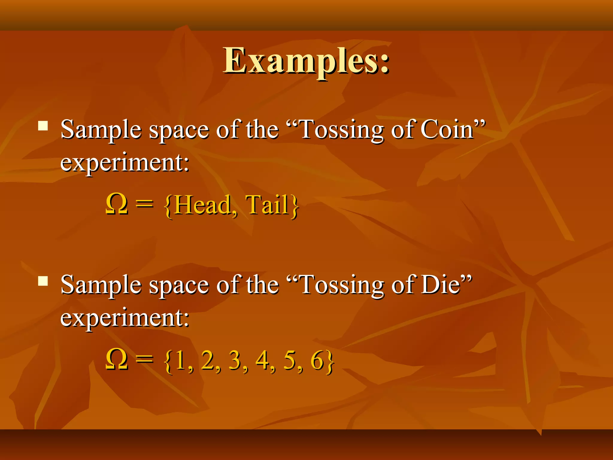
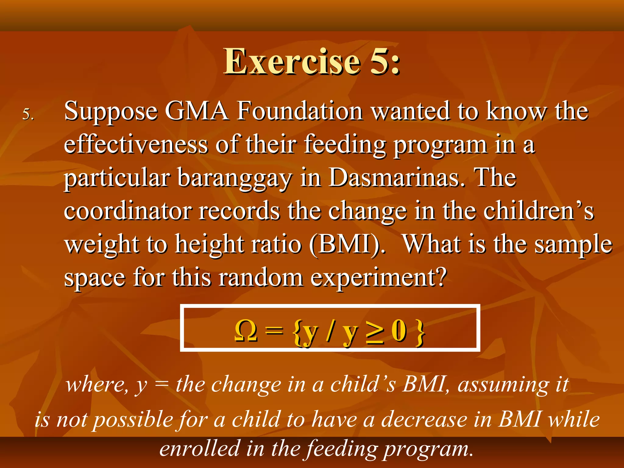
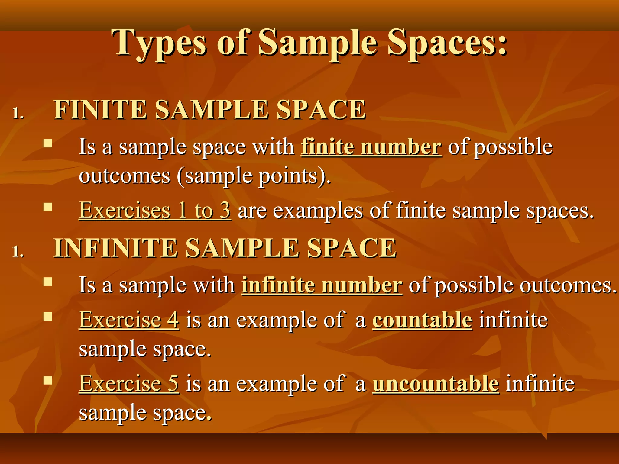
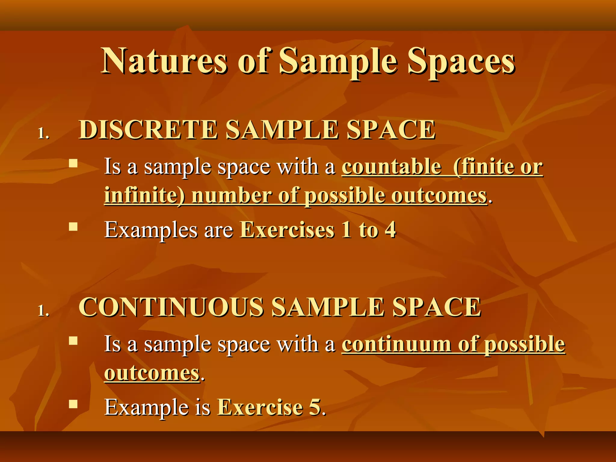
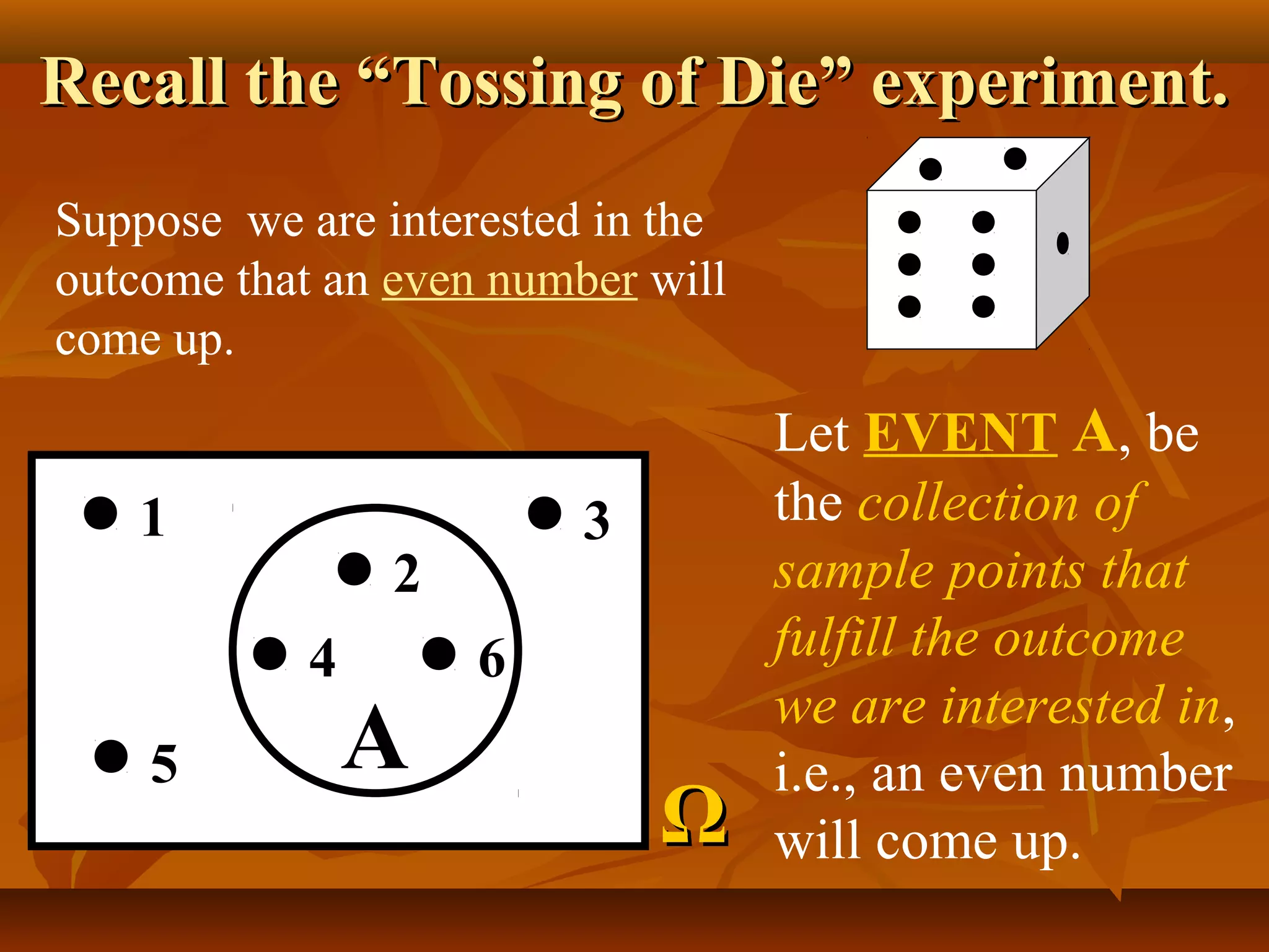
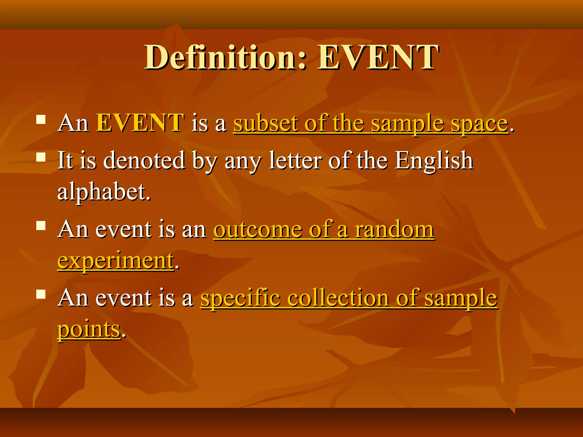
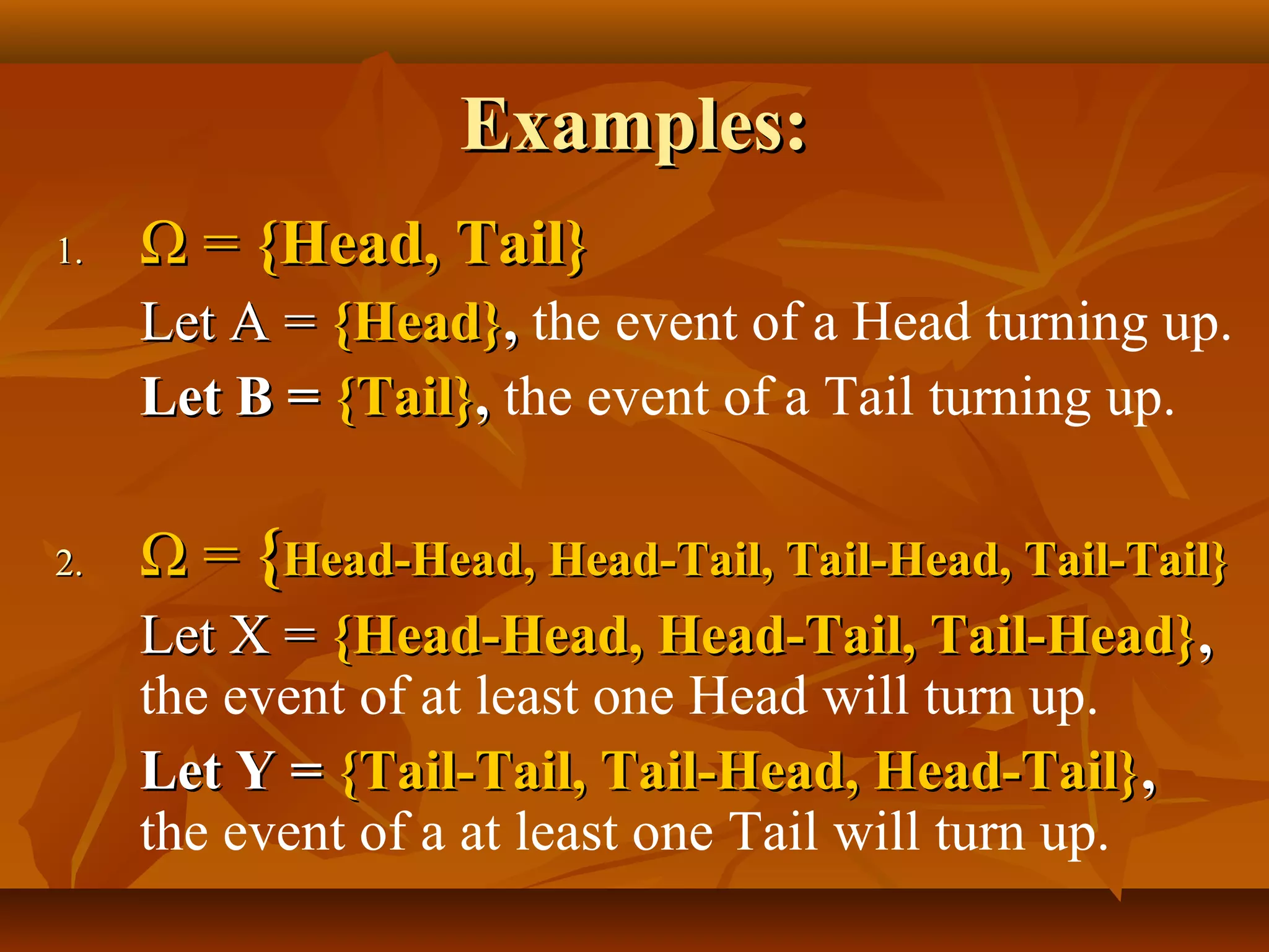
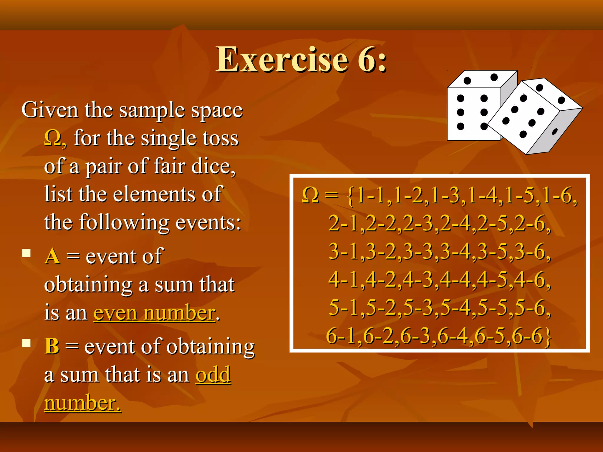
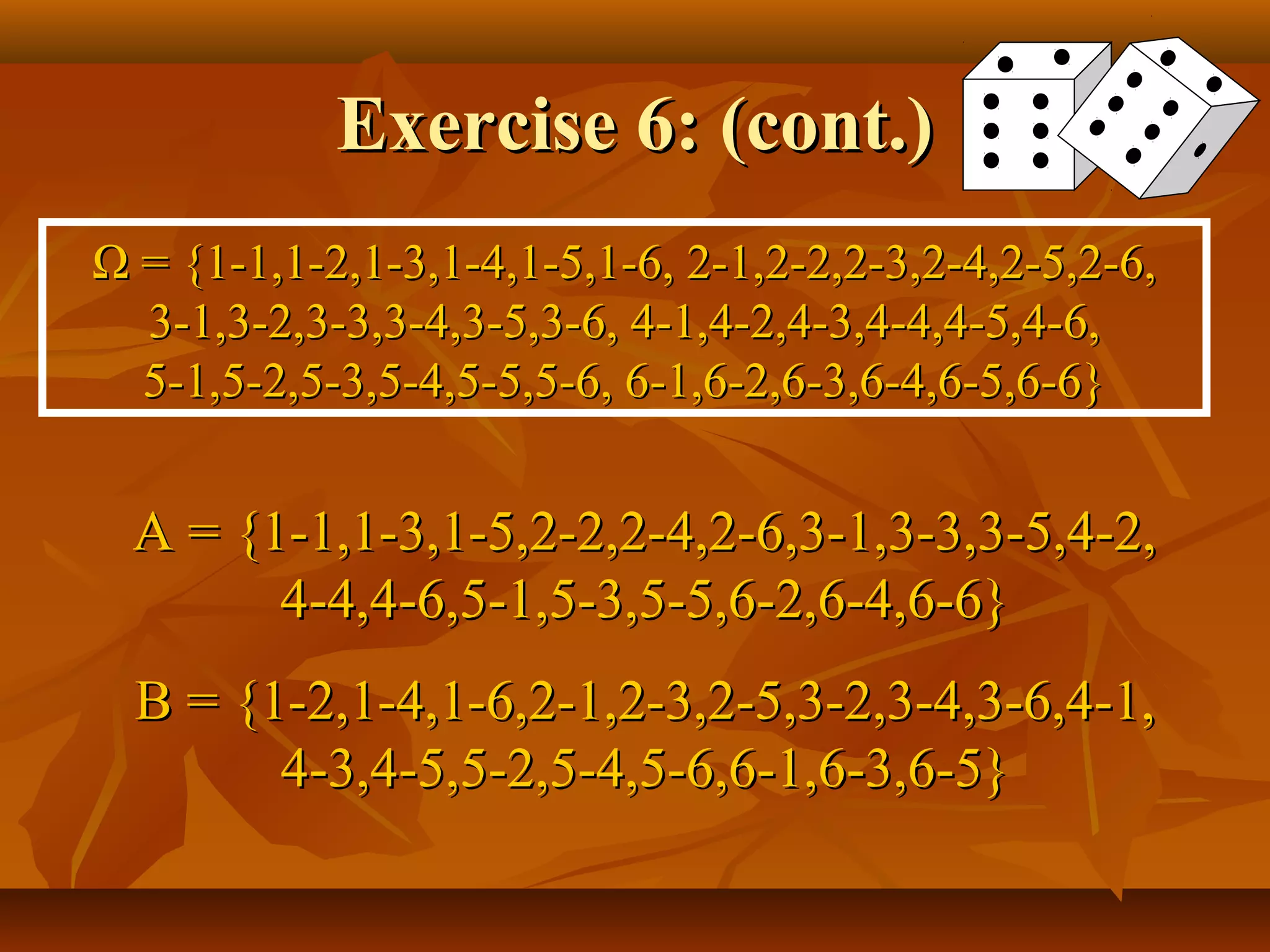
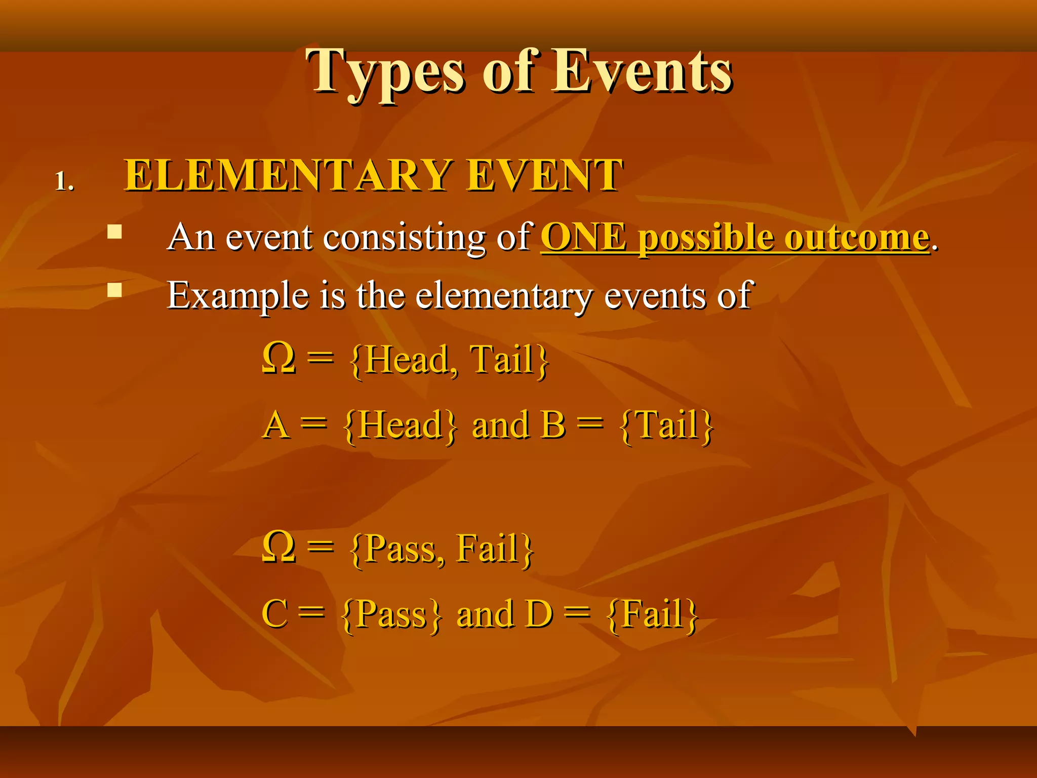
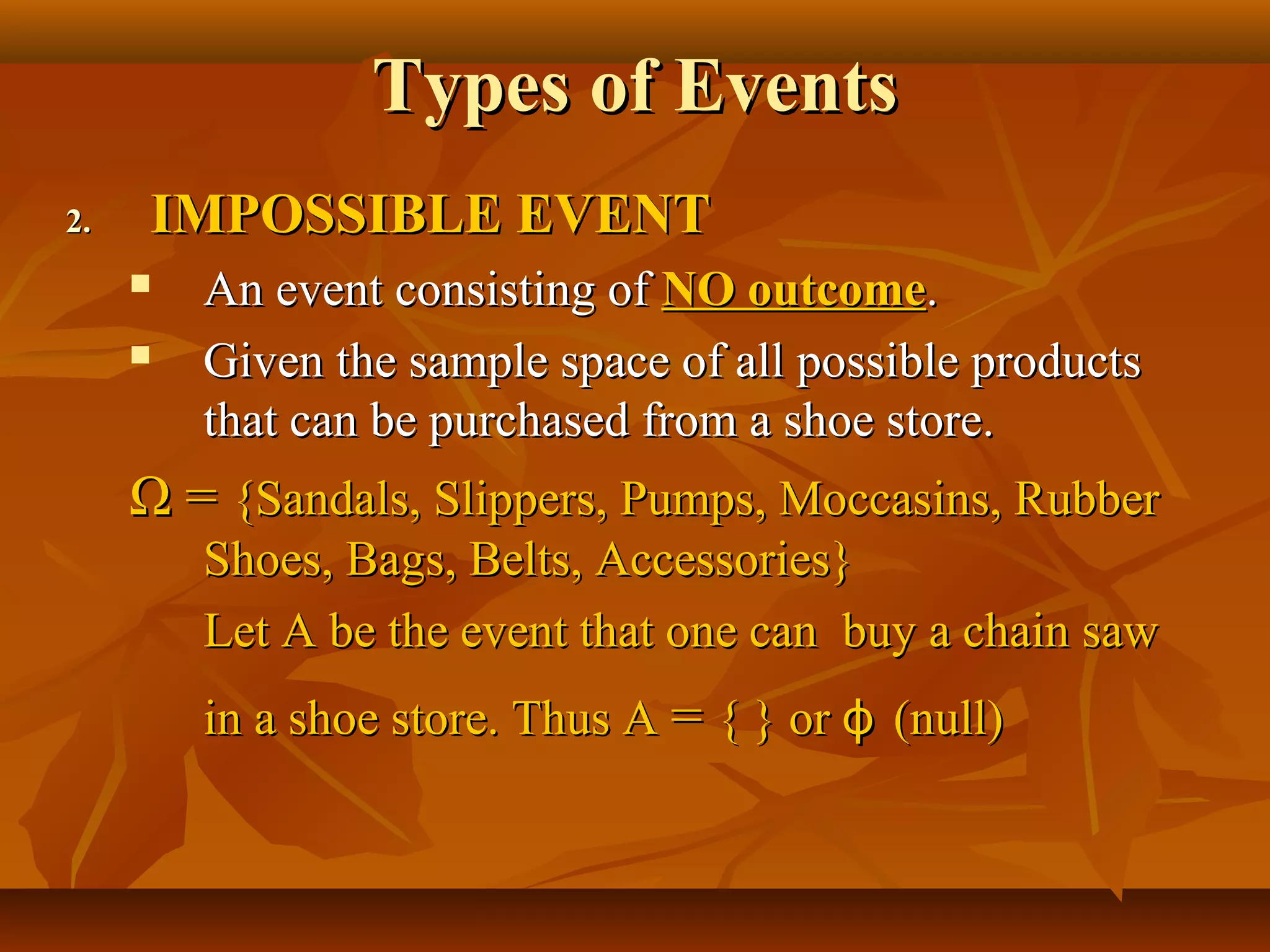
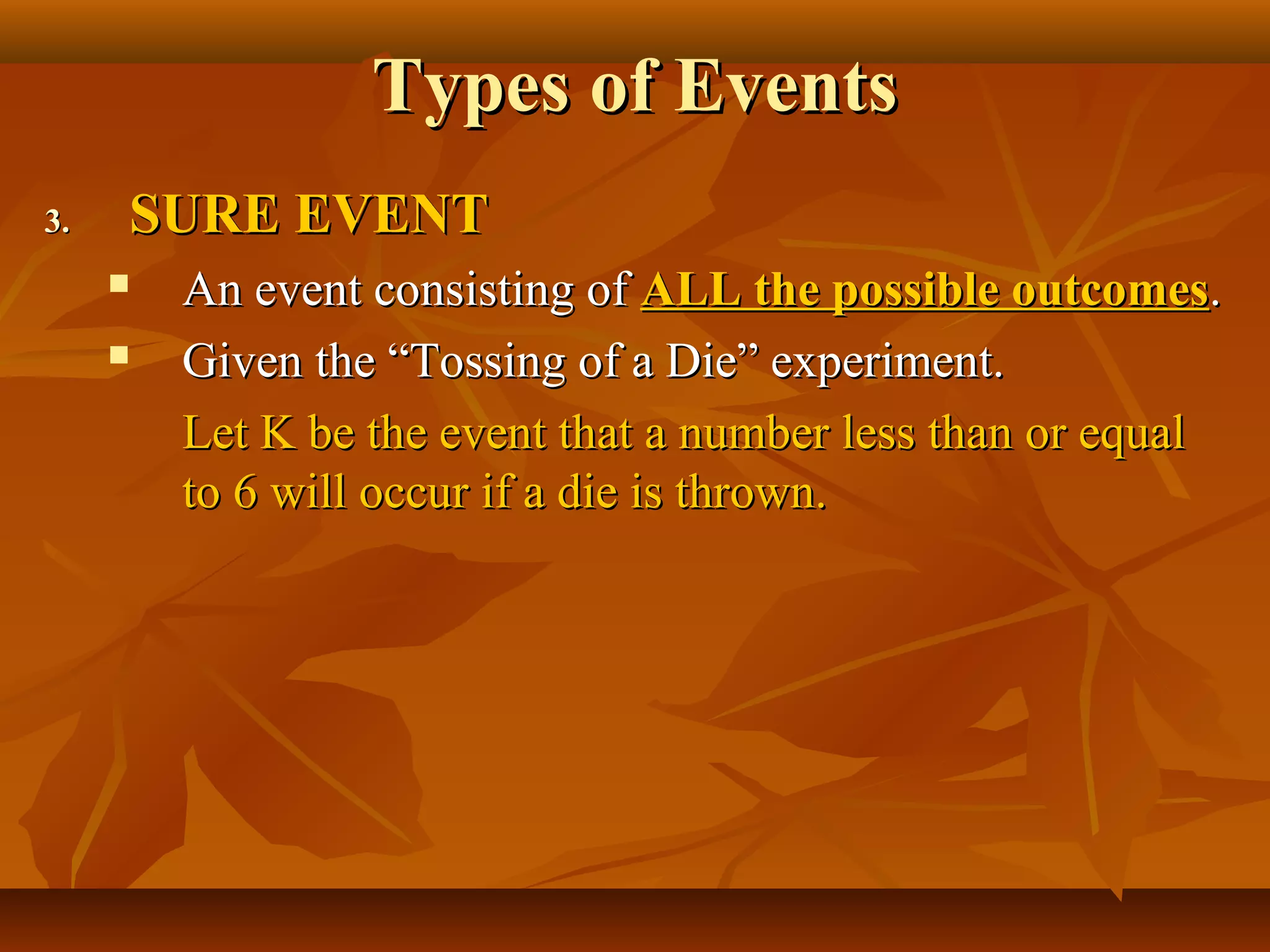
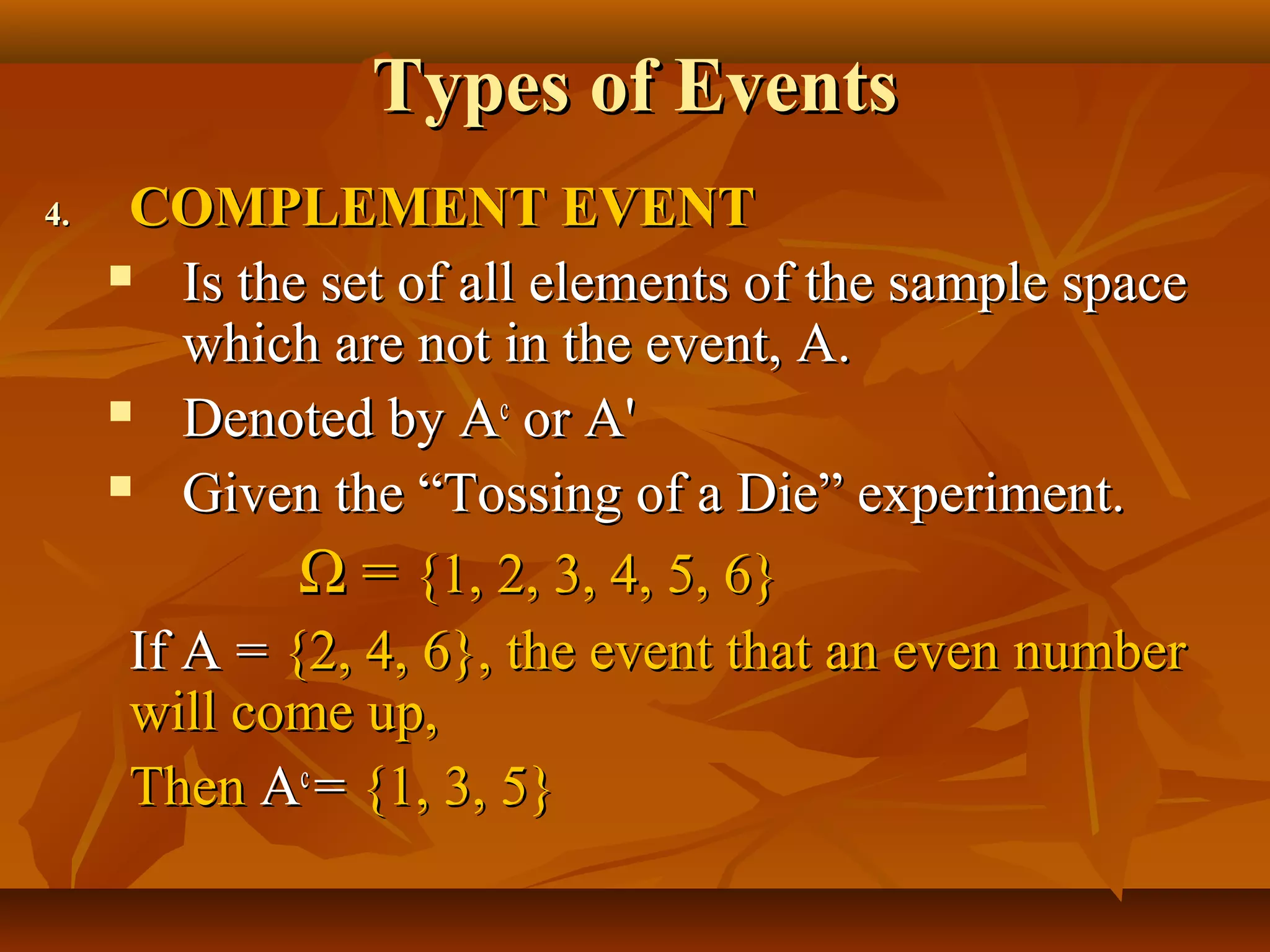
This document discusses key concepts in probability and statistics such as population, sample, random experiments, sample space, events, and types of events. It provides examples and exercises to illustrate these concepts. Specifically, it defines a random experiment as a process that can be repeated under similar conditions leading to well-defined but unpredictable outcomes. The sample space represents all possible outcomes, while an event is a subset of outcomes of interest. Events can be elementary, impossible, or sure depending on whether they consist of one, no, or all possible outcomes.

1. What have we learned so far?What have we learned so far?
POPULATION
SAMPLE
• We describe our sample using measurements and data presentation tools
• We study the sample to make inferences about the population
• What permits us to make the inferential jump from sample to population?
FDT, Graphs, Mean,
Median, Mode,
Standard Deviation,
Variance

2. PROBABILITYPROBABILITY
POPULATION
SAMPLE
 In probability, we use theIn probability, we use the
population information to inferpopulation information to infer
the probable nature of thethe probable nature of the
sample.sample.

3. Example: TOSSING A COINExample: TOSSING A COIN
 Suppose a coin is tossed onceSuppose a coin is tossed once
and the up face is recordedand the up face is recorded
 The result we see andThe result we see and
recorded is called anrecorded is called an
OBSERVATION oror
MEASUREMENT
 The process of making an
observation is called an
EXPERIMENT.

4. Definition:Definition:
RANDOM EXPERIMENTRANDOM EXPERIMENT
 Is aIs a processprocess oror procedureprocedure,, repeatable underrepeatable under
basically the same conditionbasically the same condition (this repetition(this repetition
is commonly called ais commonly called a TRIALTRIAL)), leading to, leading to well-well-
defined outcomesdefined outcomes..
 It isIt is randomrandom because we can never tell inbecause we can never tell in
advance what the outcome/realization is goingadvance what the outcome/realization is going
to be, even if we can specify what the possibleto be, even if we can specify what the possible
outcomes are.outcomes are.

5. Example: TOSSING A DIEExample: TOSSING A DIE
 Consider the simpleConsider the simple
random experiment ofrandom experiment of
tossing a die andtossing a die and
observing the numberobserving the number
on the up face.on the up face.
 There are sixThere are six basic
possible outcomes toto
this random experiment.this random experiment.
1.1. Observe aObserve a 11
2.2. Observe aObserve a 22
3.3. Observe aObserve a 33
4.4. Observe aObserve a 44
5.5. Observe aObserve a 55
6.6. Observe aObserve a 66

6. Definitions:Definitions:
SAMPLE POINT & SAMPLE SPACESAMPLE POINT & SAMPLE SPACE
 AA SAMPLE POINT is the most basicis the most basic
outcome of a random experiment.outcome of a random experiment.
 TheThe SAMPLE SPACE is the set of allis the set of all
possible outcomes of a randompossible outcomes of a random
experiment. It isexperiment. It is denoted by the Greekdenoted by the Greek
letter omega (letter omega (ΩΩ) or S) or S. This is also known. This is also known
as theas the universal setuniversal set..

7. Examples:Examples:
 Sample space of the “Tossing of Coin”Sample space of the “Tossing of Coin”
experiment:experiment:
ΩΩ == {Head, Tail}{Head, Tail}
 Sample spaceSample space of the “Tossing of Die”of the “Tossing of Die”
experiment:experiment:
ΩΩ == {1, 2, 3, 4, 5, 6}{1, 2, 3, 4, 5, 6}

8. Exercise 1:Exercise 1:
1.1. Two coins are tossed, and their up faces areTwo coins are tossed, and their up faces are
recorded. What is the sample space for thisrecorded. What is the sample space for this
experiment?experiment?
Coin 1Coin 1 Coin 2Coin 2
HeadHead HeadHead
TailTail HeadHead
HeadHead TailTail
TailTail TailTail
ΩΩ = {HH, TH, HT, TT}= {HH, TH, HT, TT}

9. Exercise 2:Exercise 2:
2.2. Suppose a pair of dice is tossed . What is the sampleSuppose a pair of dice is tossed . What is the sample
space for this experiment?space for this experiment?
ΩΩ = {1-1,1-2,1-3,1-4,1-5,1-6,= {1-1,1-2,1-3,1-4,1-5,1-6,
2-1,2-2,2-3,2-4,2-5,2-6,2-1,2-2,2-3,2-4,2-5,2-6,
3-1,3-2,3-3,3-4,3-5,3-6,3-1,3-2,3-3,3-4,3-5,3-6,
4-1,4-2,4-3,4-4,4-5,4-6,4-1,4-2,4-3,4-4,4-5,4-6,
5-1,5-2,5-3,5-4,5-5,5-6,5-1,5-2,5-3,5-4,5-5,5-6,
6-1,6-2,6-3,6-4,6-5,6-6}6-1,6-2,6-3,6-4,6-5,6-6}

10. Exercise 3:Exercise 3:
3.3. A sociologist wants to determine the gender ofA sociologist wants to determine the gender of
the first two children of families with at least twothe first two children of families with at least two
(2) children in a baranggay in Dasmarinas,(2) children in a baranggay in Dasmarinas,
Cavite. He then observes and records the genderCavite. He then observes and records the gender
of the first 2 children of these families.of the first 2 children of these families.
ΩΩ == {MM, MF, FM, FF}{MM, MF, FM, FF}
where, M represents Male and F represents Female

11. Exercise 4:Exercise 4:
4.4. Consider the experiment of recording theConsider the experiment of recording the
number of customers placing their order atnumber of customers placing their order at
the “Drive Thru” of a particular McDonald’sthe “Drive Thru” of a particular McDonald’s
branch per day. What is the sample space forbranch per day. What is the sample space for
this random experiment?this random experiment?
ΩΩ == {0, 1, 2, 3, 4, 5, …}{0, 1, 2, 3, 4, 5, …}

12. Exercise 5:Exercise 5:
5.5. Suppose GMA Foundation wanted to know theSuppose GMA Foundation wanted to know the
effectiveness of their feeding program in aeffectiveness of their feeding program in a
particular baranggay in Dasmarinas. Theparticular baranggay in Dasmarinas. The
coordinator records the change in the children’scoordinator records the change in the children’s
weight to height ratio (BMI). What is the sampleweight to height ratio (BMI). What is the sample
space for this random experiment?space for this random experiment?
ΩΩ == {y / y{y / y ≥ 0≥ 0 }}
where, y = the change in a child’s BMI, assuming it
is not possible for a child to have a decrease in BMI while
enrolled in the feeding program.

13. Types of Sample Spaces:Types of Sample Spaces:
1.1. FINITE SAMPLE SPACEFINITE SAMPLE SPACE
 Is a sample space withIs a sample space with finite numberfinite number of possibleof possible
outcomes (sample points).outcomes (sample points).
 Exercises 1 to 3Exercises 1 to 3 are examples of finite sample spaces.are examples of finite sample spaces.
1.1. INFINITE SAMPLE SPACEINFINITE SAMPLE SPACE
 Is a sample withIs a sample with infinite numberinfinite number of possible outcomes.of possible outcomes.
 Exercise 4Exercise 4 is an example of ais an example of a countablecountable infiniteinfinite
sample space.sample space.
 Exercise 5Exercise 5 is an example of ais an example of a uncountableuncountable infiniteinfinite
sample spacesample space..

14. Natures of Sample SpacesNatures of Sample Spaces
1.1. DISCRETE SAMPLE SPACEDISCRETE SAMPLE SPACE
 Is a sample space with aIs a sample space with a countable (finite orcountable (finite or
infinite) number of possible outcomesinfinite) number of possible outcomes..
 Examples areExamples are Exercises 1 to 4Exercises 1 to 4
1.1. CONTINUOUS SAMPLE SPACECONTINUOUS SAMPLE SPACE
 Is a sample space with aIs a sample space with a continuum of possiblecontinuum of possible
outcomesoutcomes..
 Example isExample is Exercise 5Exercise 5..

15. Recall the “Tossing of Die” experiment.Recall the “Tossing of Die” experiment.
Suppose we are interested in the
outcome that an even number will
come up.
1
5
3
2
4 6
A
ΩΩ
Let EVENT A, be
the collection of
sample points that
fulfill the outcome
we are interested in,
i.e., an even number
will come up.

16. Definition: EVENTDefinition: EVENT
 AnAn EVENTEVENT is ais a subset of the sample spacesubset of the sample space..
 It is denoted by any letter of the EnglishIt is denoted by any letter of the English
alphabet.alphabet.
 An event is anAn event is an outcome of a randomoutcome of a random
experimentexperiment..
 An event is aAn event is a specific collection of samplespecific collection of sample
pointspoints..

17. Examples:Examples:
1.1. ΩΩ == {Head, Tail}{Head, Tail}
Let A =Let A = {Head}{Head},, the event of a Head turning up.
Let B =Let B = {Tail}{Tail},, the event of a Tail turning up.
2.2. ΩΩ == {{Head-Head, Head-Tail, Tail-Head, Tail-Tail}Head-Head, Head-Tail, Tail-Head, Tail-Tail}
Let X =Let X = {Head-Head, Head-Tail, Tail-Head}{Head-Head, Head-Tail, Tail-Head},,
the event of at least one Head will turn up.
Let Y =Let Y = {Tail-Tail, Tail-Head, Head-Tail}{Tail-Tail, Tail-Head, Head-Tail},,
the event of a at least one Tail will turn up.

18. Exercise 6:Exercise 6:
Given the sample spaceGiven the sample space
ΩΩ,, for the single tossfor the single toss
of a pair of fair dice,of a pair of fair dice,
list the elements oflist the elements of
the following events:the following events:
 AA = event of= event of
obtaining a sum thatobtaining a sum that
is anis an even numbereven number..
 BB = event of obtaining= event of obtaining
a sum that is ana sum that is an oddodd
number.number.
ΩΩ = {1-1,1-2,1-3,1-4,1-5,1-6,= {1-1,1-2,1-3,1-4,1-5,1-6,
2-1,2-2,2-3,2-4,2-5,2-6,2-1,2-2,2-3,2-4,2-5,2-6,
3-1,3-2,3-3,3-4,3-5,3-6,3-1,3-2,3-3,3-4,3-5,3-6,
4-1,4-2,4-3,4-4,4-5,4-6,4-1,4-2,4-3,4-4,4-5,4-6,
5-1,5-2,5-3,5-4,5-5,5-6,5-1,5-2,5-3,5-4,5-5,5-6,
6-1,6-2,6-3,6-4,6-5,6-6}6-1,6-2,6-3,6-4,6-5,6-6}

19. Exercise 6: (cont.)Exercise 6: (cont.)
ΩΩ = {1-1,1-2,1-3,1-4,1-5,1-6, 2-1,2-2,2-3,2-4,2-5,2-6,= {1-1,1-2,1-3,1-4,1-5,1-6, 2-1,2-2,2-3,2-4,2-5,2-6,
3-1,3-2,3-3,3-4,3-5,3-6, 4-1,4-2,4-3,4-4,4-5,4-6,3-1,3-2,3-3,3-4,3-5,3-6, 4-1,4-2,4-3,4-4,4-5,4-6,
5-1,5-2,5-3,5-4,5-5,5-6, 6-1,6-2,6-3,6-4,6-5,6-6}5-1,5-2,5-3,5-4,5-5,5-6, 6-1,6-2,6-3,6-4,6-5,6-6}
A = {1-1,1-3,1-5,2-2,2-4,2-6,3-1,3-3,3-5,4-2,A = {1-1,1-3,1-5,2-2,2-4,2-6,3-1,3-3,3-5,4-2,
4-4,4-6,5-1,5-3,5-5,6-2,6-4,6-6}4-4,4-6,5-1,5-3,5-5,6-2,6-4,6-6}
B = {1-2,1-4,1-6,2-1,2-3,2-5,3-2,3-4,3-6,4-1,B = {1-2,1-4,1-6,2-1,2-3,2-5,3-2,3-4,3-6,4-1,
4-3,4-5,5-2,5-4,5-6,6-1,6-3,6-5}4-3,4-5,5-2,5-4,5-6,6-1,6-3,6-5}

20. Types of EventsTypes of Events
1.1. ELEMENTARY EVENTELEMENTARY EVENT
 An event consisting ofAn event consisting of ONE possible outcomeONE possible outcome..
 Example is the elementary events ofExample is the elementary events of
ΩΩ == {Head, Tail}{Head, Tail}
AA == {Head} and B{Head} and B == {Tail}{Tail}
ΩΩ == {Pass, Fail}{Pass, Fail}
CC == {Pass} and D{Pass} and D == {Fail}{Fail}

21. Types of EventsTypes of Events
2.2. IMPOSSIBLE EVENTIMPOSSIBLE EVENT
 An event consisting ofAn event consisting of NO outcomeNO outcome..
 Given the sample space of all possible productsGiven the sample space of all possible products
that can be purchased from a shoe store.that can be purchased from a shoe store.
ΩΩ == {Sandals, Slippers, Pumps, Moccasins, Rubber{Sandals, Slippers, Pumps, Moccasins, Rubber
Shoes, Bags, Belts, Accessories}Shoes, Bags, Belts, Accessories}
Let A be the event that one can buy a chain sawLet A be the event that one can buy a chain saw
in a shoe store. Thus Ain a shoe store. Thus A == { } or{ } or ϕϕ (null)(null)

22. Types of EventsTypes of Events
3.3. SURE EVENTSURE EVENT
 An event consisting ofAn event consisting of ALL the possible outcomesALL the possible outcomes..
 Given the “Tossing of a Die” experiment.Given the “Tossing of a Die” experiment.
Let K be the event that a number less than or equalLet K be the event that a number less than or equal
to 6 will occur if a die is thrown.to 6 will occur if a die is thrown.

23. Types of EventsTypes of Events
4.4. COMPLEMENT EVENTCOMPLEMENT EVENT
 Is the set of all elements of the sample spaceIs the set of all elements of the sample space
which are not in the event, A.which are not in the event, A.
 Denoted by ADenoted by Acc
or Aor A''
 Given the “Tossing of a Die” experiment.Given the “Tossing of a Die” experiment.
ΩΩ == {1, 2, 3, 4, 5, 6}{1, 2, 3, 4, 5, 6}
If A =If A = {2, 4, 6}, the event that an even number{2, 4, 6}, the event that an even number
will come up,will come up,
ThenThen AAcc
== {1, 3, 5}{1, 3, 5}

24. Operations On EventsOperations On Events
1.1. INTERSECTION of 2 events A and B, denoted byINTERSECTION of 2 events A and B, denoted by
AA∩B, is the event containing all elements that are∩B, is the event containing all elements that are
common to events A and B.common to events A and B.
Example:Example:
ΩΩ == {a, b, c, d, e, f}{a, b, c, d, e, f}
A = {a, b, c, d}A = {a, b, c, d}
B = {c, d, e, f}B = {c, d, e, f}
A ∩ B = {c, d}A ∩ B = {c, d}
ΩΩ ∩ A = {a, b, c, d}∩ A = {a, b, c, d}

25. Definition:Definition:
MUTUALLY EXCLUSIVE EVENTSMUTUALLY EXCLUSIVE EVENTS
 Two events are mutually exclusive if theyTwo events are mutually exclusive if they
cannot both occur simultaneously.cannot both occur simultaneously.
 That is, AThat is, A∩B = { } or∩B = { } or ϕϕ
 Example Let C = {1, 2, 3} and D = {a, b, c}Example Let C = {1, 2, 3} and D = {a, b, c}
ThenThen CC∩D = { }∩D = { }

26. Operations On EventsOperations On Events
2.2. UNION of 2 events A and B, denoted byUNION of 2 events A and B, denoted by
AA⋃⋃B, is the set containing all elements thatB, is the set containing all elements that
belong to A or to B or both.belong to A or to B or both.
Example:Example:
E = {1, 2, 3, 4, 5}E = {1, 2, 3, 4, 5}
F = {2, 5, 6, 7, 8}F = {2, 5, 6, 7, 8}
EE ⋃⋃ F = {1, 2, 3, 4, 5, 6, 7, 8}F = {1, 2, 3, 4, 5, 6, 7, 8}

27. Operations On EventsOperations On Events
3.3. Other OperationsOther Operations..

AA ⋃⋃ ΩΩ == ΩΩ
 AA ⋂ A' =⋂ A' = ϕϕ
 ΩΩ' =' = ϕϕ
 (A')' = A(A')' = A

AA ⋃⋃ ϕϕ = A= A

AA ⋃ A'⋃ A' == ΩΩ

ϕϕ'' == ΩΩ