Downloaded 55 times
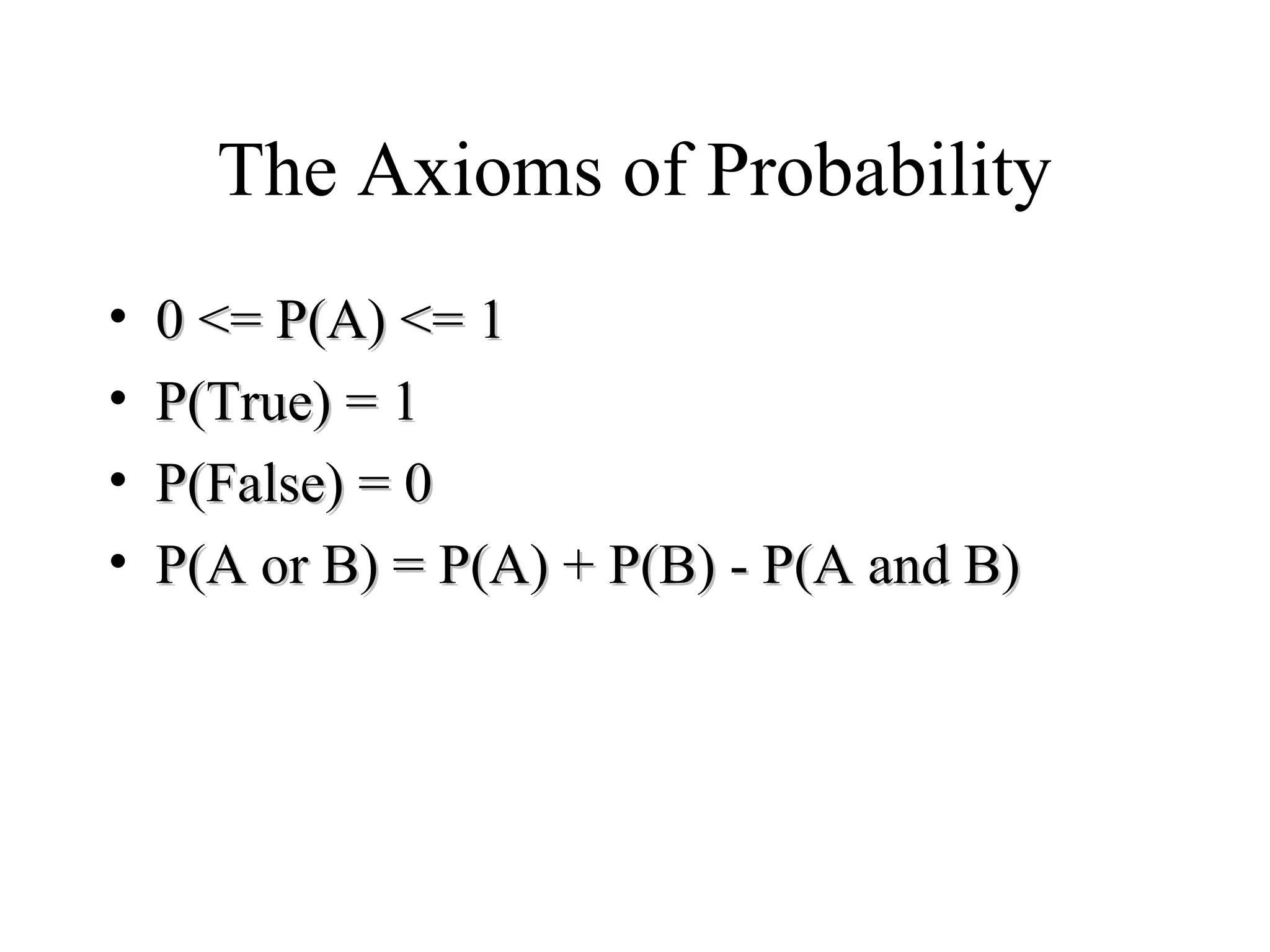
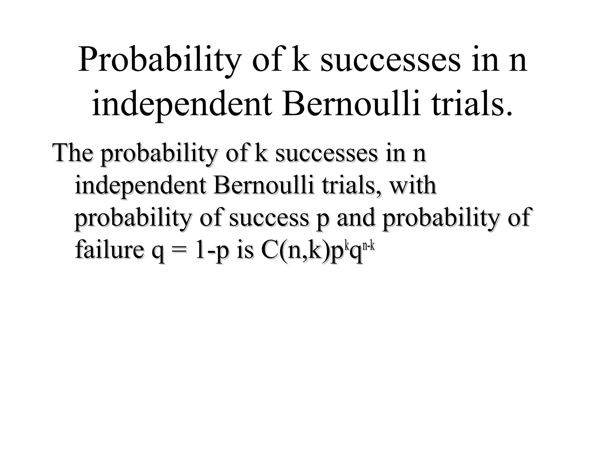
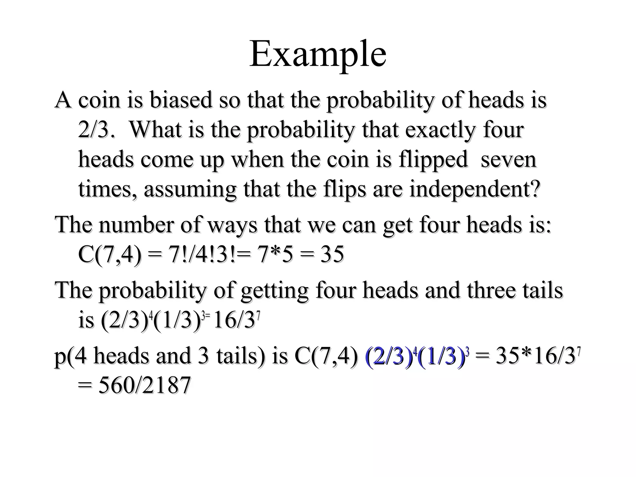
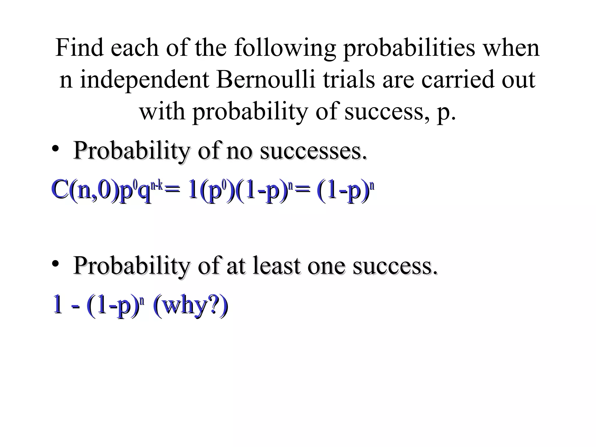
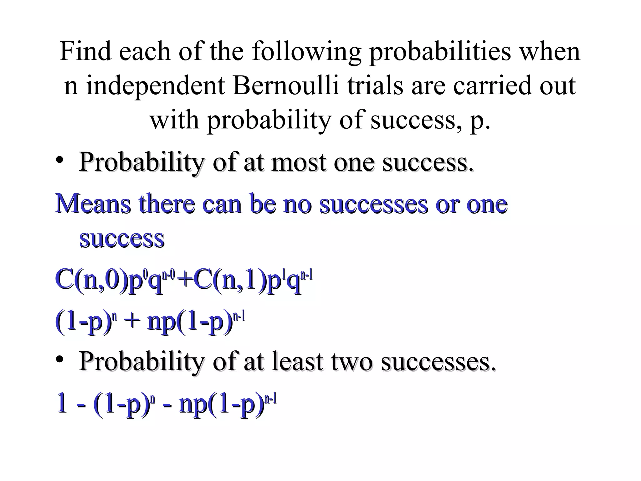
![Module #19 – Probability
Experiments & Sample Spaces
• A (stochastic)A (stochastic) experimentexperiment is any process by whichis any process by which
a given random variablea given random variable VV gets assigned somegets assigned some
particularparticular value, and where this value is notvalue, and where this value is not
necessarily known in advance.necessarily known in advance.
– We call it the “actual” value of the variable, asWe call it the “actual” value of the variable, as
determined by that particular experiment.determined by that particular experiment.
• TheThe sample spacesample space SS of the experiment is justof the experiment is just
the domain of the random variable,the domain of the random variable, SS = dom[= dom[VV]]..
• TheThe outcomeoutcome of the experiment is the specificof the experiment is the specific
valuevalue vvii of the random variable that is selected.of the random variable that is selected.](https://image.slidesharecdn.com/probabilitytheory1-150708103619-lva1-app6892/75/Probability-theory-5-2048.jpg)
![Module #19 – Probability
Events
• AnAn eventevent EE is any set of possible outcomes inis any set of possible outcomes in SS……
– That is,That is, EE ⊆⊆ SS == domdom[[VV]]..
• E.g., the event that “less than 50 people show up for our nextE.g., the event that “less than 50 people show up for our next
class” is represented as the setclass” is represented as the set {1, 2, …, 49}{1, 2, …, 49} of values of theof values of the
variablevariable VV = (# of people here next class)= (# of people here next class)..
• We say that eventWe say that event EE occursoccurs when the actual valuewhen the actual value
ofof VV is inis in EE, which may be written, which may be written VV∈∈EE..
– Note thatNote that VV∈∈EE denotes the proposition (of uncertaindenotes the proposition (of uncertain
truth) asserting that the actual outcome (value oftruth) asserting that the actual outcome (value of VV) will) will
be one of the outcomes in the setbe one of the outcomes in the set EE..](https://image.slidesharecdn.com/probabilitytheory1-150708103619-lva1-app6892/75/Probability-theory-6-2048.jpg)
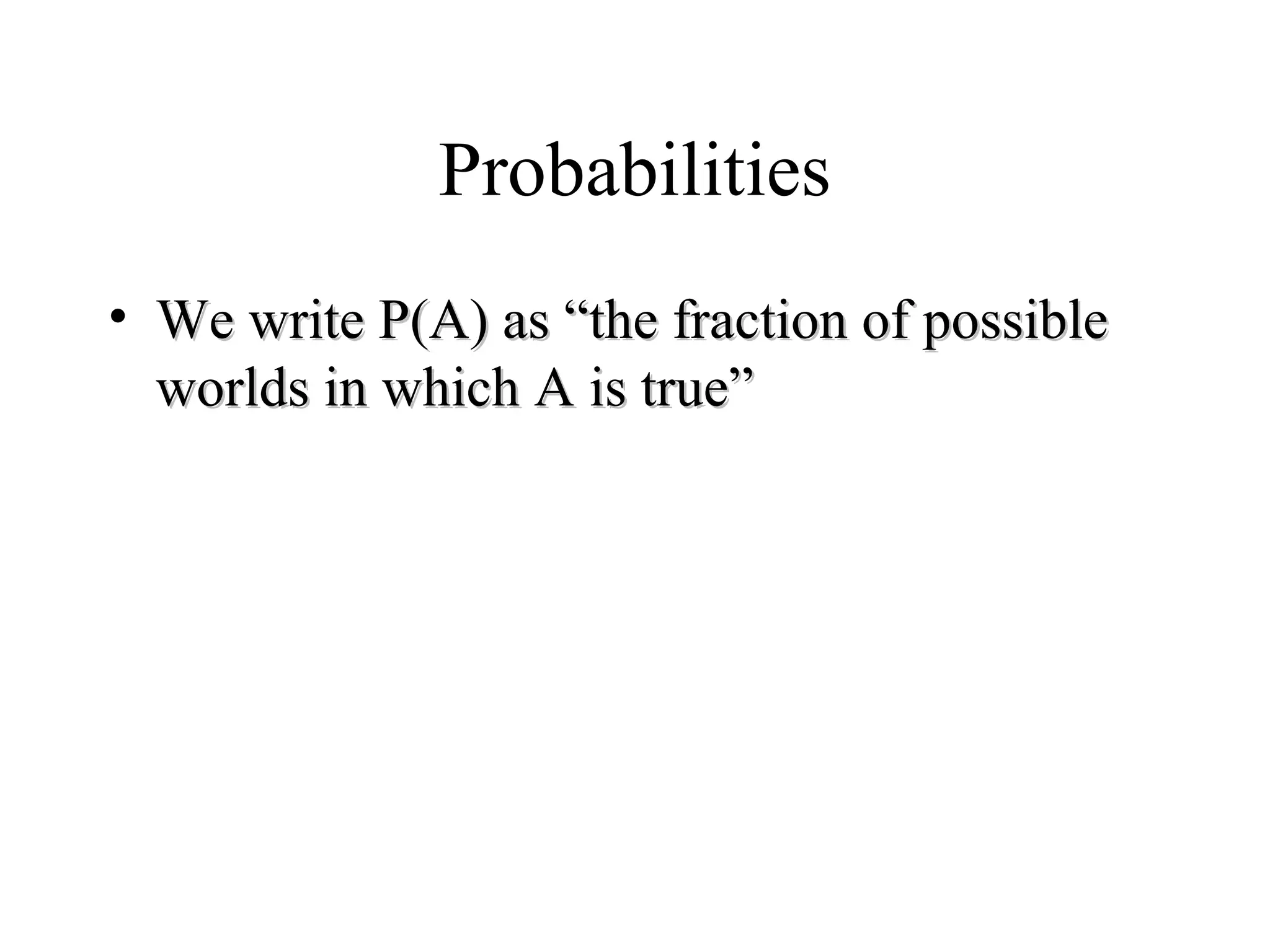
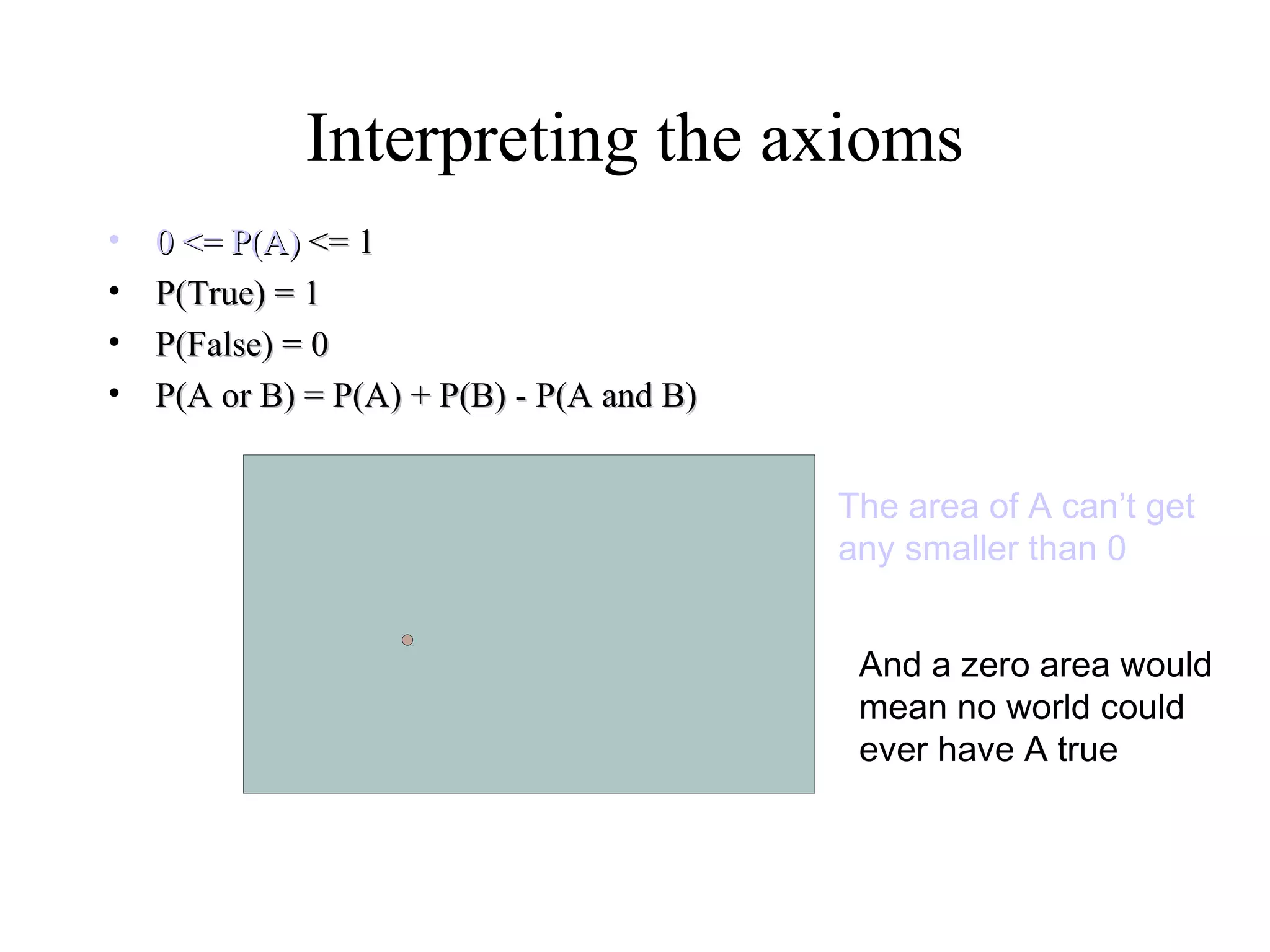
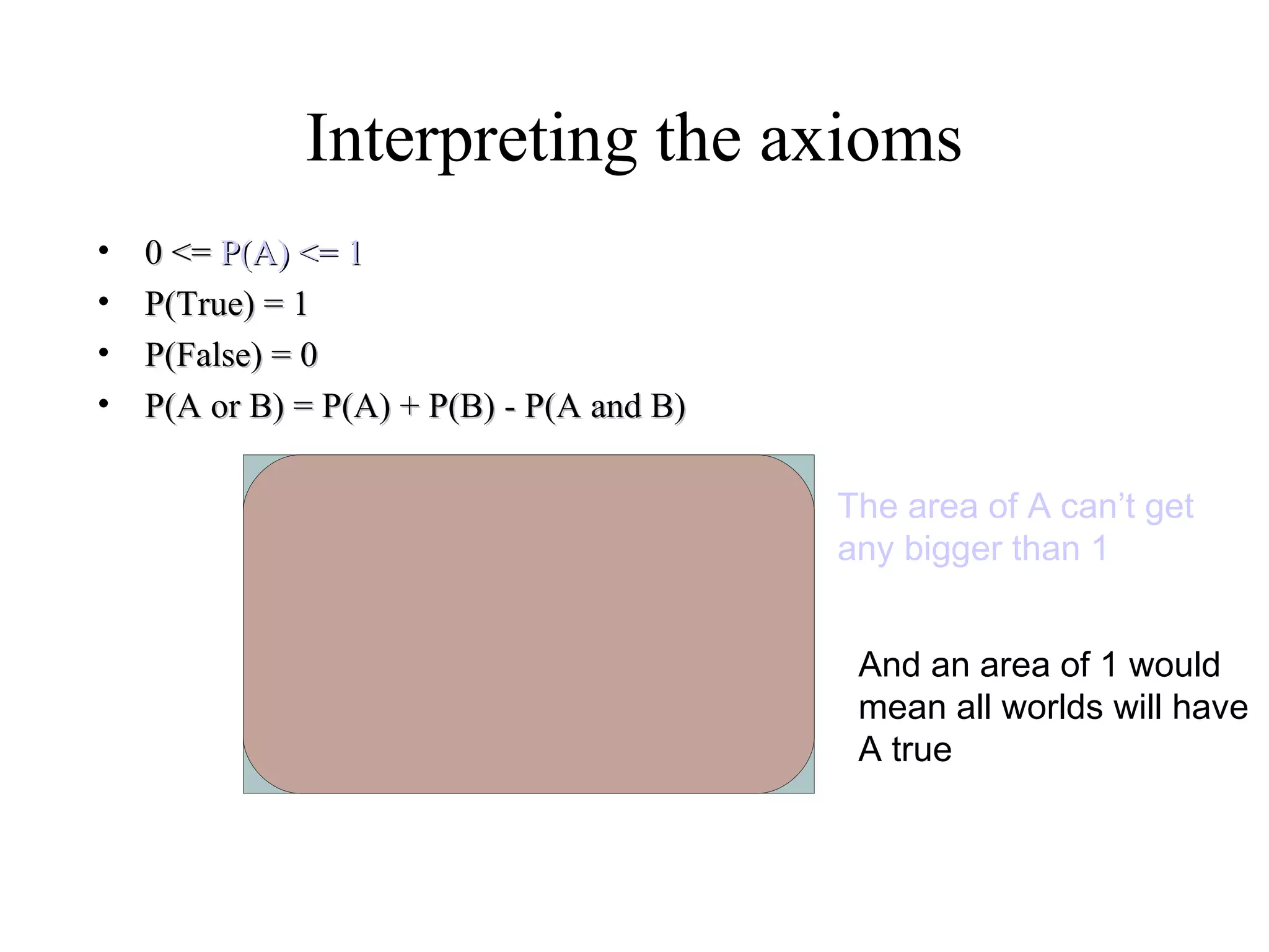
![Module #19 – Probability
Probability
• TheThe probabilityprobability pp = Pr[= Pr[EE]] ∈∈ [0,1][0,1] of an eventof an event EE isis
a real number representing our degree of certaintya real number representing our degree of certainty
thatthat EE will occur.will occur.
– IfIf Pr[Pr[EE] = 1] = 1, then, then EE is absolutely certain to occur,is absolutely certain to occur,
• thusthus VV∈∈EE has the truth valuehas the truth value TrueTrue..
– IfIf Pr[Pr[EE] = 0] = 0, then, then EE is absolutely certainis absolutely certain notnot to occur,to occur,
• thusthus VV∈∈EE has the truth valuehas the truth value FalseFalse..
– IfIf Pr[Pr[EE] =] = ½½, then we are, then we are maximally uncertainmaximally uncertain aboutabout
whetherwhether EE will occur; that is,will occur; that is,
• VV∈∈EE andand VV∉∉EE are consideredare considered equally likelyequally likely..
– How do we interpret other values ofHow do we interpret other values of pp??
Note: We could also define probabilities for more
general propositions, as well as events.](https://image.slidesharecdn.com/probabilitytheory1-150708103619-lva1-app6892/75/Probability-theory-9-2048.jpg)
![Module #19 – Probability
Probability: Frequentist Definition
• The probability of an eventThe probability of an event EE is the limit, asis the limit, as nn→∞→∞,, ofof
the fraction of times that we findthe fraction of times that we find VV∈∈EE over the courseover the course
ofof nn independent repetitions of (different instances of)independent repetitions of (different instances of)
the same experiment.the same experiment.
• Some problems with this definition:Some problems with this definition:
– It is only well-defined for experiments that can beIt is only well-defined for experiments that can be
independently repeated, infinitely many times!independently repeated, infinitely many times!
• or at least, if the experiment can be repeated in principle,or at least, if the experiment can be repeated in principle, e.g.e.g., over, over
some hypothetical ensemble of (say) alternate universes.some hypothetical ensemble of (say) alternate universes.
– It can never be measured exactly in finite time!It can never be measured exactly in finite time!
• Advantage:Advantage: It’s an objective, mathematical definition.It’s an objective, mathematical definition.
n
n
E EV
n
∈
∞→
≡ lim:]Pr[](https://image.slidesharecdn.com/probabilitytheory1-150708103619-lva1-app6892/75/Probability-theory-11-2048.jpg)
![Module #19 – Probability
Probability: Bayesian Definition
• Suppose a rational, profit-maximizing entitySuppose a rational, profit-maximizing entity RR isis
offered a choice between two rewards:offered a choice between two rewards:
– WinningWinning $1$1 if and only if the eventif and only if the event EE actually occurs.actually occurs.
– ReceivingReceiving pp dollars (wheredollars (where pp∈∈[0,1][0,1]) unconditionally.) unconditionally.
• IfIf RR can honestly state that he is completelycan honestly state that he is completely
indifferent between these two rewards, then we sayindifferent between these two rewards, then we say
thatthat RR’s probability for’s probability for EE isis pp, that is,, that is, PrPrRR[[EE] :] :≡≡ pp..
• Problem:Problem: It’s a subjective definition; depends on theIt’s a subjective definition; depends on the
reasonerreasoner RR, and his knowledge, beliefs, & rationality., and his knowledge, beliefs, & rationality.
– The version above additionally assumes that the utility ofThe version above additionally assumes that the utility of
money is linear.money is linear.
• This assumption can be avoided by using “utils” (utility units)This assumption can be avoided by using “utils” (utility units)
instead of dollars.instead of dollars.](https://image.slidesharecdn.com/probabilitytheory1-150708103619-lva1-app6892/75/Probability-theory-12-2048.jpg)
![Module #19 – Probability
Probability: Laplacian Definition
• First, assume that all individual outcomes in theFirst, assume that all individual outcomes in the
sample space aresample space are equally likelyequally likely to each otherto each other……
– Note that this term still needs an operational definition!Note that this term still needs an operational definition!
• Then, the probability of any eventThen, the probability of any event EE is given by,is given by,
Pr[Pr[EE] = |] = |EE|/||/|SS||.. Very simple!Very simple!
• Problems:Problems: Still needs a definition forStill needs a definition for equally likelyequally likely,,
and depends on the existence ofand depends on the existence of somesome finite samplefinite sample
spacespace SS in which all outcomes inin which all outcomes in SS are, in fact,are, in fact,
equally likely.equally likely.](https://image.slidesharecdn.com/probabilitytheory1-150708103619-lva1-app6892/75/Probability-theory-13-2048.jpg)
![Module #19 – Probability
Probability: Axiomatic Definition
• LetLet pp be any total functionbe any total function pp::SS→[0,1]→[0,1] such thatsuch that
∑∑ss pp((ss) = 1) = 1..
• Such aSuch a pp is called ais called a probability distributionprobability distribution..
• Then, theThen, the probability under pprobability under p
of any eventof any event EE⊆⊆SS is just:is just:
• Advantage:Advantage: Totally mathematically well-defined!Totally mathematically well-defined!
– This definition can even be extended to apply to infiniteThis definition can even be extended to apply to infinite
sample spaces, by changingsample spaces, by changing ∑∑→→∫∫, and calling, and calling pp aa
probability density functionprobability density function or a probabilityor a probability measuremeasure..
• Problem:Problem: Leaves operational meaning unspecified.Leaves operational meaning unspecified.
∑∈
≡
Es
spEp )(:][](https://image.slidesharecdn.com/probabilitytheory1-150708103619-lva1-app6892/75/Probability-theory-14-2048.jpg)
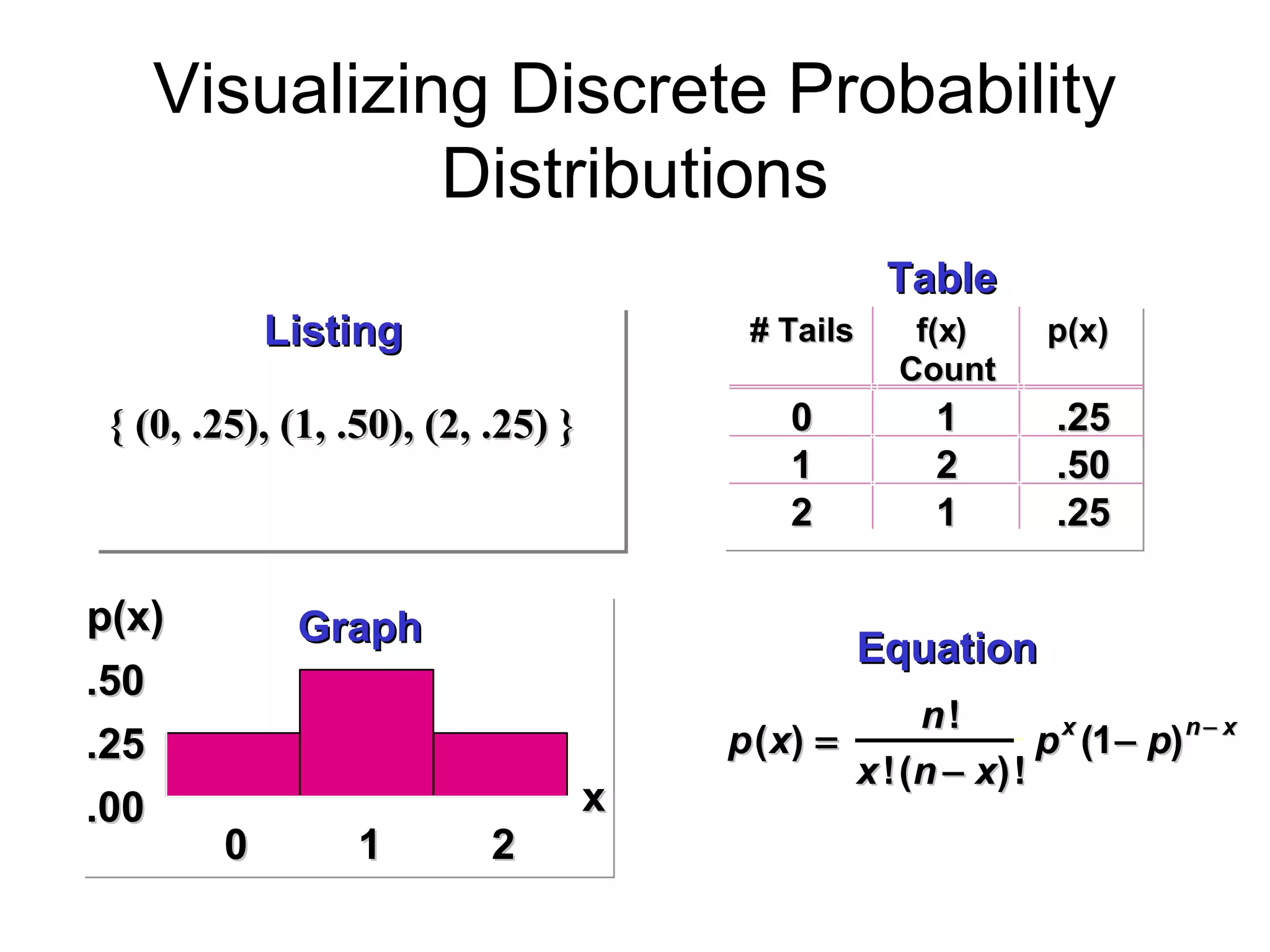
![Module #19 – Probability
Discrete Probability Distribution
( also called probability mass function (pmf) )
1.1.List of All possible [List of All possible [xx,, pp((xx)] pairs)] pairs
– xx = Value of Random Variable (Outcome)= Value of Random Variable (Outcome)
– pp((xx) = Probability Associated with Value) = Probability Associated with Value
2.2.Mutually Exclusive (No Overlap)Mutually Exclusive (No Overlap)
3.3.Collectively Exhaustive (Nothing Left Out)Collectively Exhaustive (Nothing Left Out)
4. 04. 0 ≤≤ pp((xx)) ≤≤ 11
5.5. ∑∑ pp((xx) = 1) = 1](https://image.slidesharecdn.com/probabilitytheory1-150708103619-lva1-app6892/75/Probability-theory-28-2048.jpg)
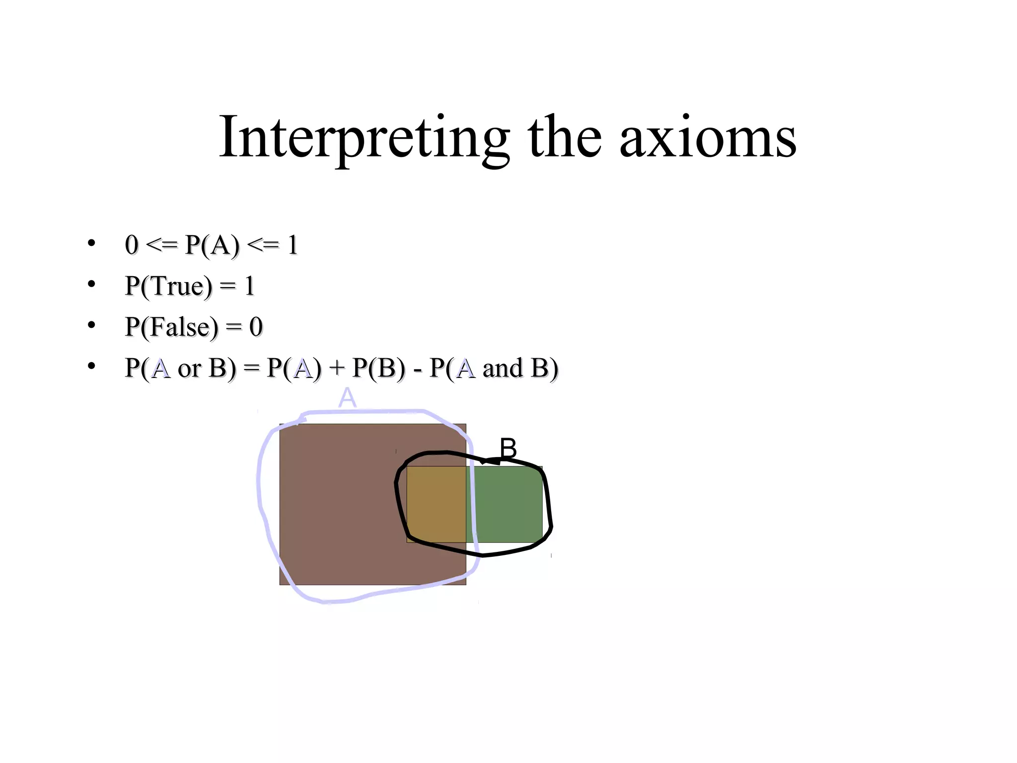
![Module #19 – Probability
Mutually Exclusive Events
• Two eventsTwo events EE11,, EE22 are calledare called mutuallymutually
exclusiveexclusive if they are disjoint:if they are disjoint: EE11∩∩EE22 == ∅∅
– Note that two mutually exclusive eventsNote that two mutually exclusive events cannotcannot
both occurboth occur in the same instance of a givenin the same instance of a given
experiment.experiment.
• For mutually exclusive events,For mutually exclusive events,
Pr[Pr[EE11 ∪∪ EE22] = Pr[] = Pr[EE11] + Pr[] + Pr[EE22]]..](https://image.slidesharecdn.com/probabilitytheory1-150708103619-lva1-app6892/75/Probability-theory-30-2048.jpg)
![Module #19 – Probability
Exhaustive Sets of Events
• A setA set EE = {= {EE11,, EE22, …}, …} of events in the sampleof events in the sample
spacespace SS is calledis called exhaustiveexhaustive iff .iff .
• An exhaustive setAn exhaustive set EE of events that are all mutuallyof events that are all mutually
exclusive with each other has the property thatexclusive with each other has the property that
SEi =
.1]Pr[ =∑ iE](https://image.slidesharecdn.com/probabilitytheory1-150708103619-lva1-app6892/75/Probability-theory-31-2048.jpg)

![Module #19 – Probability
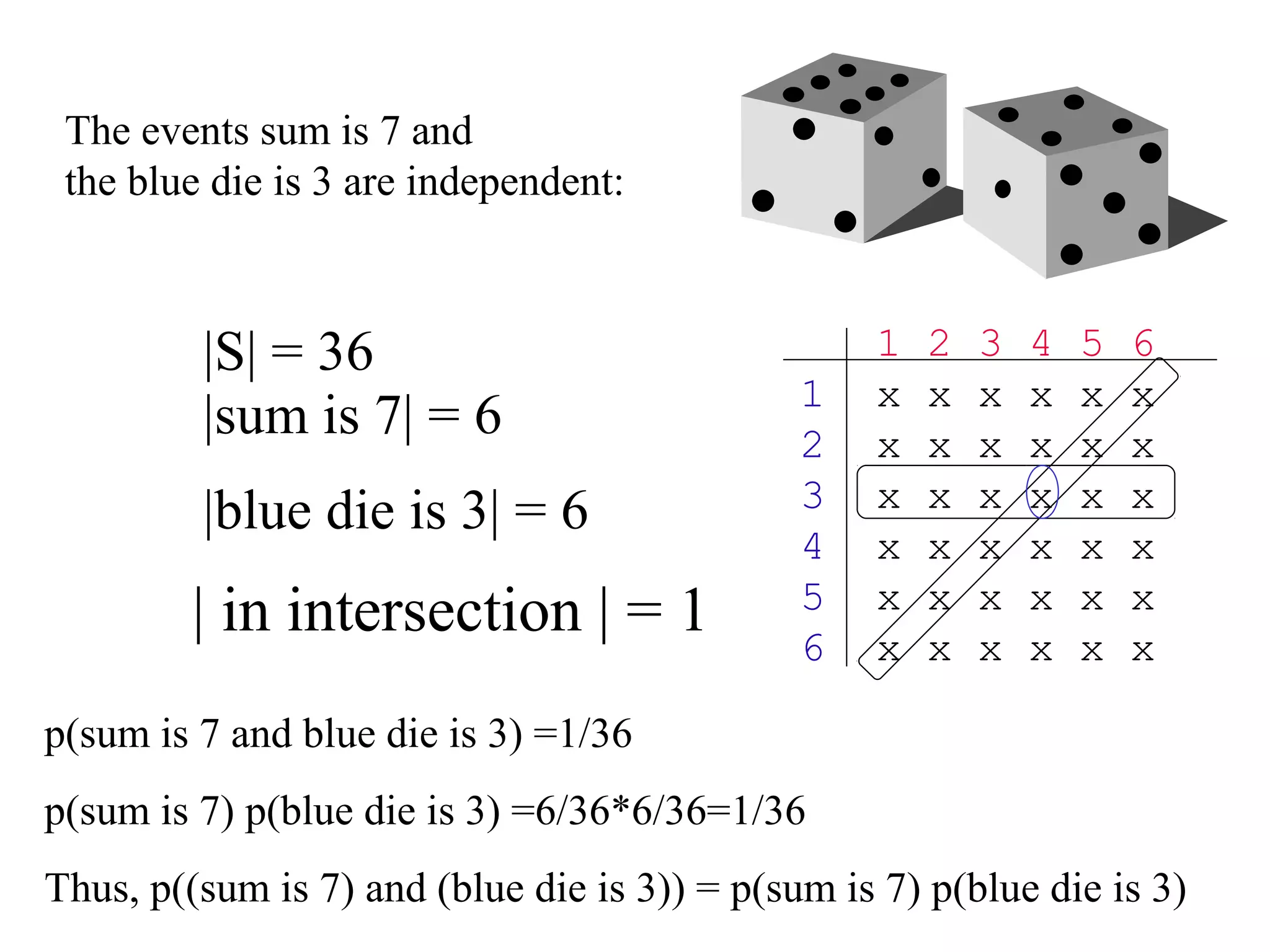
Independent Events
• Two events E,F are called independent if
Pr[E∩F] = Pr[E]·Pr[F].
• Relates to the product rule for the number
of ways of doing two independent tasks.
• Example: Flip a coin, and roll a die.
Pr[(coin shows heads) ∩ (die shows 1)] =
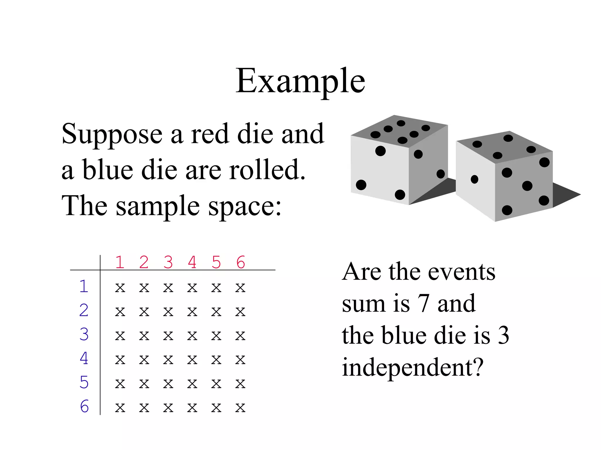
Pr[coin is heads] × Pr[die is 1] = ½×1/6 =1/12.](https://image.slidesharecdn.com/probabilitytheory1-150708103619-lva1-app6892/75/Probability-theory-41-2048.jpg)
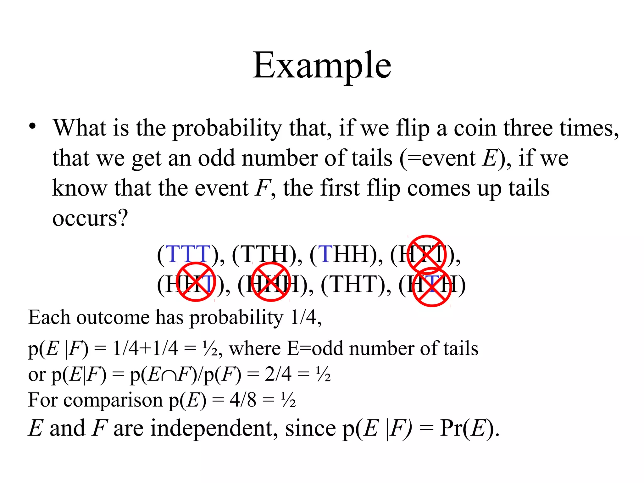
![Module #19 – Probability
Conditional Probability
• LetLet EE,,FF be any events such thatbe any events such that Pr[Pr[FF]>0]>0..
• Then, theThen, the conditional probabilityconditional probability ofof EE givengiven FF,,
writtenwritten Pr[Pr[EE||FF]], is defined as, is defined as
Pr[Pr[EE||FF] :] :≡≡ Pr[Pr[EE∩∩FF]/Pr[]/Pr[FF]]..
• This is what our probability thatThis is what our probability that EE would turn outwould turn out
to occur should be, if we are givento occur should be, if we are given onlyonly thethe
information thatinformation that FF occurs.occurs.
• IfIf EE andand FF are independent thenare independent then Pr[Pr[EE||FF] = Pr[] = Pr[EE]]..
Pr[Pr[EE||FF] = Pr[] = Pr[EE∩∩FF]/Pr[]/Pr[FF] = Pr[] = Pr[EE]]×Pr[×Pr[FF]/Pr[]/Pr[FF] = Pr[] = Pr[EE]]](https://image.slidesharecdn.com/probabilitytheory1-150708103619-lva1-app6892/75/Probability-theory-44-2048.jpg)
![Module #19 – Probability
• Suppose I choose a single letter out of the 26-letter English
alphabet, totally at random.
– Use the Laplacian assumption on the sample space {a,b,..,z}.
– What is the (prior) probability
that the letter is a vowel?
• Pr[Vowel] = __ / __ .
• Now, suppose I tell you that the
letter chosen happened to be in
the first 9 letters of the alphabet.
– Now, what is the conditional (or
posterior) probability that the letter
is a vowel, given this information?
• Pr[Vowel | First9] = ___ / ___ .
Conditional Probability Example
a
b c
d
e f
g
h
i
j
k
l
mn
o
p q
r
s
t
u
v
w
x
y
z
1st
9
lettersvowels
Sample Space S](https://image.slidesharecdn.com/probabilitytheory1-150708103619-lva1-app6892/75/Probability-theory-46-2048.jpg)
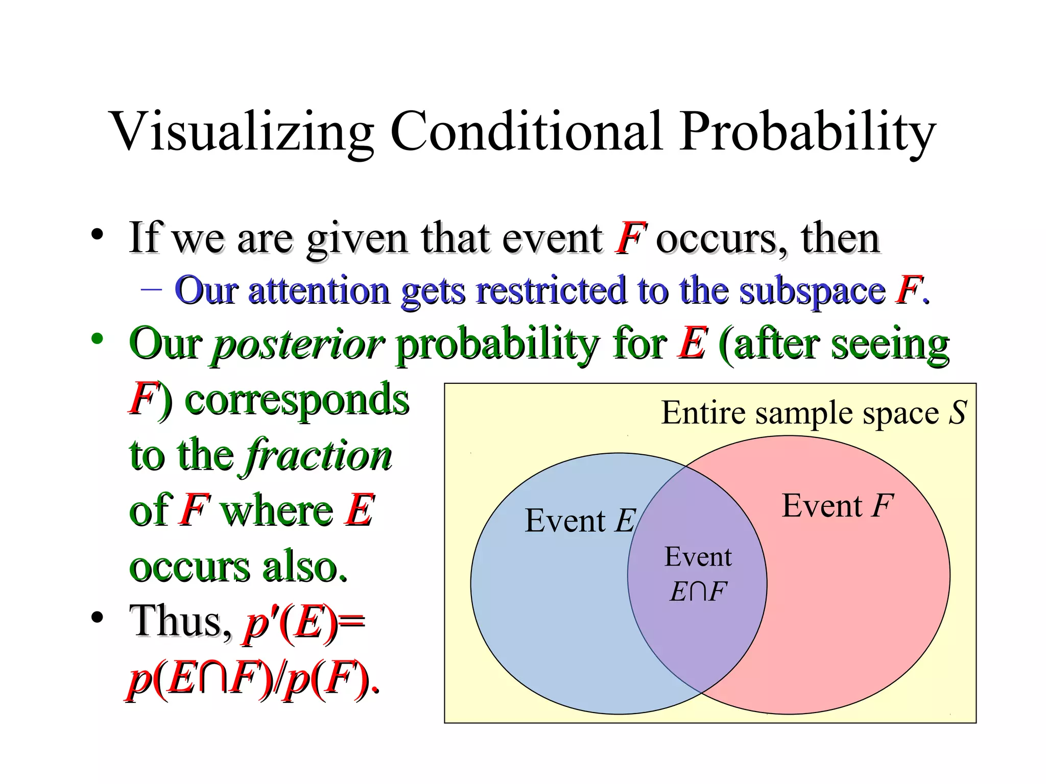
![Module #19 – Probability
Prior and Posterior Probability
• Suppose that, before you are given any information about the
outcome of an experiment, your personal probability for an
event E to occur is p(E) = Pr[E].
– The probability of E in your original probability distribution p is called
the prior probability of E.
• This is its probability prior to obtaining any information about the outcome.
• Now, suppose someone tells you that some event F (which may
overlap with E) actually occurred in the experiment.
– Then, you should update your personal probability for event E to occur,
to become p′(E) = Pr[E|F] = p(E∩F)/p(F).
• The conditional probability of E, given F.
– The probability of E in your new probability distribution p′ is called the
posterior probability of E.
• This is its probability after learning that event F occurred.
• After seeing F, the posterior distribution p′ is defined by letting
p′(v) = p({v}∩F)/p(F) for each individual outcome v∈S.](https://image.slidesharecdn.com/probabilitytheory1-150708103619-lva1-app6892/75/Probability-theory-48-2048.jpg)

This document provides an overview of key concepts in probability theory: - An experiment yields possible outcomes called a sample space. Events are subsets of outcomes. Random variables assign values to outcomes. - Probability is a measure of certainty that an event will occur, ranging from 0 (impossible) to 1 (certain). It can be defined in different ways. - The frequentist definition is the limit of relative frequencies of an event over many trials. The Bayesian definition is a degree of belief in an event. The Laplacian definition assumes all outcomes are equally likely initially. - Examples demonstrate random variables, events, and calculating probabilities based on the sample space and outcomes of an experiment. Key terms like sample space, event,


![ch_5-8_probability155[1].ppt](https://cdn.slidesharecdn.com/ss_thumbnails/ch5-8probability1551-231116061842-b428d0bc-thumbnail.jpg?width=640&height=640&fit=bounds)