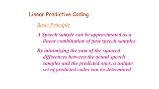
Downloaded 56 times

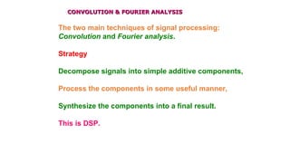
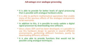
![SIGNAL
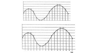
Continuous signals x(t)
A description of how one parameter varies with
another parameter
Discrete signals x[n]](https://image.slidesharecdn.com/speechtechnology-basics-170105105857/85/Speech-technology-basics-4-320.jpg)
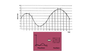
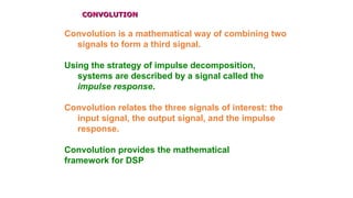
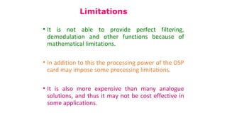
![DIGITAL SIGNAL
DIGITAL signals x[n]
Discrete signals x[n]](https://image.slidesharecdn.com/speechtechnology-basics-170105105857/85/Speech-technology-basics-5-320.jpg)

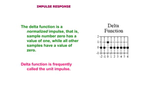
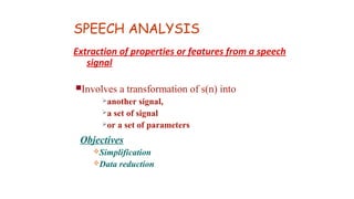
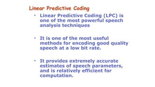
![Fourier Decomposition
Any N point signal can be
decomposed into N/2 signals,
half of them sine waves and half
of them cosine waves.
The lowest frequency cosine
wave (called in this xC0 [n]
illustration), makes zero complete
cycles over the N samples, i.e., it
is a DC signal.](https://image.slidesharecdn.com/speechtechnology-basics-170105105857/85/Speech-technology-basics-21-320.jpg)
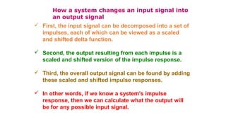
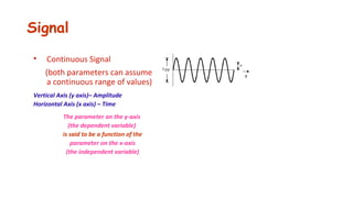
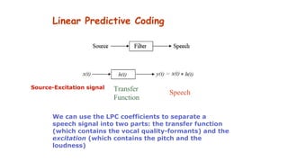
![Fourier Decomposition
The next cosine components: , ,
and , make 1, 2, xC1 [n] xC2 [n] xC3
[n] and 3 complete cycles over the
N samples, respectively.
Since the frequency of each
component is fixed, the only
thing that changes for different
signals being decomposed is the
amplitude of each of the sine and
cosine waves.](https://image.slidesharecdn.com/speechtechnology-basics-170105105857/85/Speech-technology-basics-22-320.jpg)
![IMPULSE RESPONSEIMPULSE RESPONSE
Impulse response is the signal
that exits a system when a
delta function (unit impulse)
is the input.
If two systems are different in
any way, they will have
different impulse
responses.
Just as the input and
output signals are often
called x[n] y[n] and , the
impulse response is
usually given the name is
h[n]](https://image.slidesharecdn.com/speechtechnology-basics-170105105857/85/Speech-technology-basics-26-320.jpg)
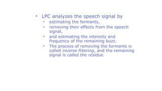
![IMPULSE RESPONSEIMPULSE RESPONSE
• Any impulse can be
represented as a shifted and
scaled delta function.
• Consider a signal, , composed
of all zeros except sample
number 8, a[n] which has a
value of -3.
• This is the same as a delta
function shifted to the right by 8
samples, and multiplied by -3.
• In equation form: a[n] = -3δ[n-8]](https://image.slidesharecdn.com/speechtechnology-basics-170105105857/85/Speech-technology-basics-27-320.jpg)
![IMPULSE RESPONSEIMPULSE RESPONSE
If the input to a system is
an impulse, such as , -3δ[n-
8] what is the system's
output?
Scaling and shifting the
input results in an identical
scaling and shifting of the
output.](https://image.slidesharecdn.com/speechtechnology-basics-170105105857/85/Speech-technology-basics-28-320.jpg)
![IMPULSE RESPONSEIMPULSE RESPONSE
If -3δ[n-8] results in h[n] , it
follows that -3δ[n-8] results in
-3h[n-8] h[n]
In words, the output is a
version of the impulse
response that has been
shifted and scaled by the
same amount as the delta
function on the input.
If you know a system's
impulse response, you
immediately know how it will
react to any impulse.](https://image.slidesharecdn.com/speechtechnology-basics-170105105857/85/Speech-technology-basics-29-320.jpg)
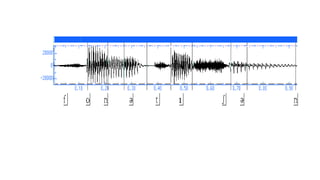
![Short Time Autocorrelation
Speech signal of s(n)
Fourier transform of s(n) = S(e jw
)
Energy spectrum = [S(e jw
) ]2
[S(e jw
)]2
is called Autocorrelation of s(n)
This preserves information about
harmonic and formant amplitudes in s(n)](https://image.slidesharecdn.com/speechtechnology-basics-170105105857/85/Speech-technology-basics-45-320.jpg)
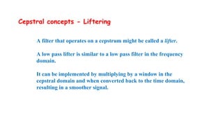
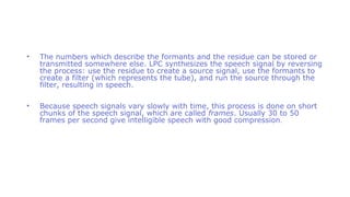

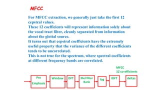
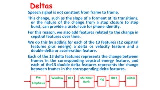
![The extraction of the cepstrum with the inverse DFT results in 12
cepstral coeffcients for each frame.
We next add a 13th
feature; the energy from the frame.
Energy correlates with phone identity and so is a useful cue for phone
detection (vowels and sibilants have more energy that stops, etc.).
The energy in a frame is the sum over time of the power of the
samples in the frame; thus, for a signal x in a window from time
sample t1 to time sample t1, the energy is
t2
Energy = ∑ x2
[t]
t=t1
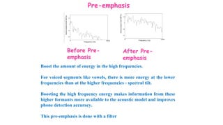
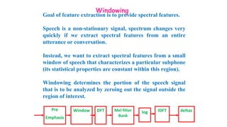
Pre
Emphasis
Window DFT Mel filter
Bank
log IDFT deltas
Energy](https://image.slidesharecdn.com/speechtechnology-basics-170105105857/85/Speech-technology-basics-78-320.jpg)


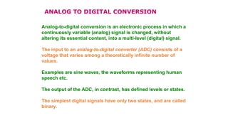
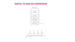
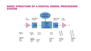
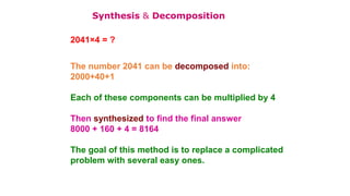
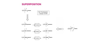
Digital signal processing (DSP) involves converting analog signals to digital signals and manipulating the digital signals using software algorithms. DSP systems use analog-to-digital conversion to convert analog signals to digital signals represented as sequences of numbers. They then process the digital signals using a digital signal processor and convert them back to analog signals using digital-to-analog conversion. Key techniques in DSP include decomposing signals into simple components, processing the components individually, and then combining the results.