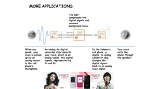
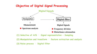
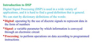
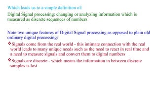
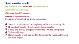
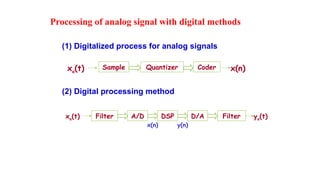
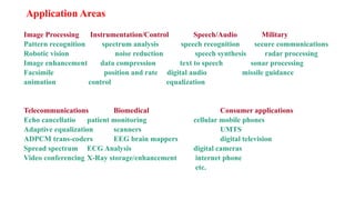
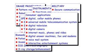
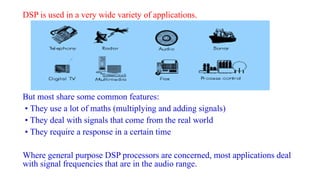
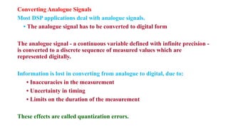
Digital Signal Processing (DSP) deals with the manipulation of discrete signals representing real-world information through a variety of applications. It is distinguished from analog systems by its versatility, repeatability, and the ability to handle signals in a precise and reprogrammable manner, addressing needs such as real-time processing and accuracy. DSP encompasses various operations including signal transformation, filtering, and analysis, and addresses challenges like quantization errors and aliased frequencies during the conversion from analog to digital forms.

1. Advanced Digital Signal Processing
Introduction to DSP
Prof. Dr. Mohammed Najm Abdullah
https://itswtech.academia.edu/MohammedAlSalam

2. Introduction to DSP
Digital Signal Processing (DSP) is used in a wide variety of
applications, and it is hard to find a good definition that is general.
We can start by dictionary definitions of the words:
Digital: operating by the use of discrete signals to represent data in
the form of numbers
Signal: a variable parameter by which information is conveyed
through an electronic circuit
Processing: to perform operations on data according to programmed
instructions

3. Which leads us to a simple definition of:
Digital Signal processing: changing or analyzing information which is
measured as discrete sequences of numbers
Note two unique features of Digital Signal processing as opposed to plain old
ordinary digital processing:
Signals come from the real world - this intimate connection with the real
world leads to many unique needs such as the need to react in real time and
a need to measure signals and convert them to digital numbers
Signals are discrete - which means the information in between discrete
samples is lost

4. Digital better than Analog
 Analog
- Aging
- Sensitivity to the environment
- Uncertain performance in production units
- Variation in performance of units
- Sensitivity analog traces on PCBs
- Effort to migrate and adopt “canned” solutions
 DSP doesn’t have these problems!

5. Variable of Signals ：
Time/Distance/Temperature/Voltage
One-dimensional Signals ： Single variable y=x(t)
Two-dimensional Signals ： Two variables
Three-dimensional Signals ： Three variables
By a signal we mean any variable that carries or contains
some kind of information that can be conveyed,
displayed or manipulated.

6. Classification of Signal
Continuous-time and discrete-time signal
Analog and digital signal (time and amplitude)
(1) Continuous-time signal ：
(2) Discrete-time signal ： Discrete variableContinuous amplitude
Time-domain discrete signals
(3) Analog Signal: Continuous variableContinuous amplitude
Speech, Television, Time-domain continuous signals
(4) Digital Signal ： Discrete variablesDiscrete amplitude
Quantized discrete-time signals

8. Examples of signals of particular interest are:
 Speech, is encountered in telephony, radio, and everyday life
 Biomedical signals, (heart signals, brain signals)
 Sound and music, as reproduced by the compact disc player
 Video and image,
 Radar signals, which are used to determine the range and bearing
of distant targets
Signal operation include:
(1) Transform, filter, inspection, spectrum analysis;
(2) Modulation and coding;
(3) Analog Signal Processing;
(4) Digital Signal Processing.

9. Basic concepts about system
(1) System
Device or technology of signal processing.
(2) Analog system
System with analog input and output.
(3) Digital system
System with digital input and output.

10. Signals and Systems
Basic model:
Input: x Output: y
10
System: h
DSP 、 FPGA 、 SOPC 、 SOC 、 Algorithm Codes

11. x y
• Given x and h, find y analysis
• Given h and y, find x control
• Given x and y, find h design or
synthesis
11
h
Three Problems

12. Processing of analog signal with digital methods
(1) Digitalized process for analog signals
Sample Quantizer Coder
xa(t) x(n)
(2) Digital processing method
A/D DSP D/A
xa(t) ya(t)
Filter
x(n) y(n)
Filter

13. SIGNAL PROCESSING METHODS
Signal processing methods have evolved in algorithmic complexity, aiming for
optimal utilization of the information in order to achieve the best performance. In
general the computational requirement of signal processing methods increases,
often exponentially, with the algorithmic complexity. However, the
implementation cost of advanced signal processing methods has been offset and
made affordable by the consistent trend in recent years of a continuing increase in
the performance, coupled with a simultaneous decrease in the cost, of signal
processing hardware.
Depending on the method used, digital signal processing algorithms can be
categorized into one or a combination of four broad categories. These are
transform-based signal processing, model-based signal processing, Bayesian
statistical signal processing and neural networks, as illustrated in Figure

15. The advantages of DSP are common to many digital systems and include:
Versatility:
• Digital systems can be reprogrammed for other applications (at least where
programmable DSP chips are used)
• Digital systems can be ported to different hardware (for example a different DSP chip
or board level product)
Repeatability:
• Digital systems can be easily duplicated
• Digital systems do not depend on strict component tolerances
• Digital system responses do not drift with temperature
Simplicity:
• Some things can be done more easily digitally than with analogue systems

16. Application Areas
Image Processing Instrumentation/Control Speech/Audio Military
Pattern recognition spectrum analysis speech recognition secure communications
Robotic vision noise reduction speech synthesis radar processing
Image enhancement data compression text to speech sonar processing
Facsimile position and rate digital audio missile guidance
animation control equalization
Telecommunications Biomedical Consumer applications
Echo cancellatio patient monitoring cellular mobile phones
Adaptive equalization scanners UMTS
ADPCM trans-coders EEG brain mappers digital television
Spread spectrum ECG Analysis digital cameras
Video conferencing X-Ray storage/enhancement internet phone
etc.

17. IMAGE PROCESSING
Pattern recognition
Robotic vision
Image enhancement
Satellite weather map
animation
INSTRUMENTATION & CONTROL
Spectrum analysis
Position and rate control
Noise reduction
Data compression
SPEECH & AUDIO
Speech recognition
Speech synthesis
Text to speech
digital audio
MILITARY
Secure communication
Radar processing
Sonar processing
Missile guidance
TELECOMMUNICATION
Echo cancellation
Adaptive equalization
Video conferencing
data communication
Biomedical
Patient monitoring
Scanners
ECG (Electrocardiograph)
X-ray storage/enhancement
Consumer applications
digital, cellar mobile phones
universal mobile telecommunication system
digital television
digital camera
internet music, phones and video
digital answer machines, fax and modems
voice mail system
interactive entertainment systems

18. DSP is used in a very wide variety of applications.
But most share some common features:
• They use a lot of maths (multiplying and adding signals)
• They deal with signals that come from the real world
• They require a response in a certain time
Where general purpose DSP processors are concerned, most applications deal
with signal frequencies that are in the audio range.

19. Converting Analogue Signals
Most DSP applications deal with analogue signals.
• The analogue signal has to be converted to digital form
The analogue signal - a continuous variable defined with infinite precision -
is converted to a discrete sequence of measured values which are
represented digitally.
Information is lost in converting from analogue to digital, due to:
• Inaccuracies in the measurement
• Uncertainty in timing
• Limits on the duration of the measurement
These effects are called quantization errors.

20. The continuous analogue signal has to be held before it can be sampled.
Otherwise, the signal would be changing during the measurement.

21. Only after it has been held can the signal be measured, and the measurement
converted to a digital value.
The sampling results in a discrete set of digital numbers that represent
measurements of the signal - usually taken at equal intervals of time.
Note that the sampling takes place after the hold. This means that we can
sometimes use a slower Analogue to Digital Converter (ADC) than might
seem required at first sight. The hold circuit must act fast - fast enough that the
signal is not changing during the time the circuit is acquiring the signal value -
but the ADC has all the time that the signal is held to make its conversion.
We don't know what we don't measure.
In the process of measuring the signal, some information is lost

23. • For periodic waveforms, the duration of the waveform
before it repeats is called the period of the waveform

24. Frequency
• The rate at which a regular vibration pattern repeats itself
(frequency = 1/period)

25. Frequency of a Waveform
• The unit for frequency is cycles/second, also called
Hertz (Hz).
• The frequency of a waveform is equal to the reciprocal
of the period.
frequency = 1/period

26. Frequency of a Waveform
• Examples:
frequency = 10 Hz
period = .1 (1/10) seconds
frequency = 100 Hz
period = .01 (1/100) seconds
frequency = 261.6 Hz
period = .0038226 (1/ 261.6) seconds

27. Waveform Sampling
• To represent waveforms on digital computers, we need to
digitize or sample the waveform.
• side effects of digitization:
• introduces some noise
• limits the maximum upper frequency range

28. Sampling Rate
• The sampling rate (SR) is the rate at which
amplitude values are digitized from the original
waveform.
• CD sampling rate (high-quality):
SR = 44,100 samples/second
• medium-quality sampling rate:
SR = 22,050 samples/second
• phone sampling rate (low-quality):
SR = 8,192 samples/second

29. Sampling Rate
• Higher sampling rates
allow the waveform to
be more accurately
represented

30. Nyquist Theorem and Aliasing
• Nyquist Theorem:
We can digitally represent only frequencies up to half the sampling rate.
• Example:
CD: SR=44,100 Hz
Nyquist Frequency = SR/2 = 22,050 Hz
• Example:
SR=22,050 Hz
Nyquist Frequency = SR/2 = 11,025 Hz

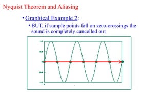
31. Nyquist Theorem and Aliasing
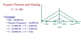
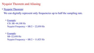
• Frequencies above Nyquist frequency "fold over"
to sound like lower frequencies.
• This fold over is called aliasing.
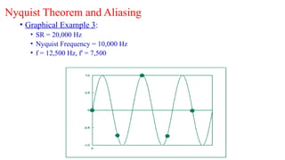
• Aliased frequency f in range [SR/2, SR] becomes
f':
f' = |f - SR|

32. Nyquist Theorem and Aliasing
f' = |f - SR|
• Example:
• SR = 20,000 Hz
• Nyquist Frequency = 10,000 Hz
• f = 12,000 Hz → f' = 8,000 Hz
• f = 18,000 Hz → f' = 2,000 Hz
• f = 20,000 Hz → f' = 0 Hz

33. Nyquist Theorem and Aliasing
• Graphical Example 1a:
• SR = 20,000 Hz
• Nyquist Frequency = 10,000 Hz
• f = 2,500 Hz (no aliasing)

34. Nyquist Theorem and Aliasing
• Graphical Example 1b:
• SR = 20,000 Hz
• Nyquist Frequency = 10,000 Hz
• f = 5,000 Hz (no aliasing)
(left and right figures have same frequency, but have different sampling points)

35. Nyquist Theorem and Aliasing
• Graphical Example 2:
• SR = 20,000 Hz
• Nyquist Frequency = 10,000 Hz
• f = 10,000 Hz (no aliasing)

36. Nyquist Theorem and Aliasing
•Graphical Example 2:
• BUT, if sample points fall on zero-crossings the
sound is completely cancelled out

37. Nyquist Theorem and Aliasing
• Graphical Example 3:
• SR = 20,000 Hz
• Nyquist Frequency = 10,000 Hz
• f = 12,500 Hz, f' = 7,500

43. When you
speak, your
voice is picked
up by an
analog sensor
in the cell
phone’s
microphone
An analog-to-digital
converter chip converts
your voice, which is an
analog signal, into digital
signals, represented by
1s and 0s.
The DSP
compresses the
digital signals and
removes
background noise.
In the listener’s
cell phone, a
digital-to-analog
converter chip
changes the
digital signals
back to an analog
voice signal.
Your voice
exits the
phone through
the speaker.
MORE APPLICATIONS

44. A MP3 Player

45. (3) Noise process  Digital filter
(1) Selective of A/D  Signal representation - Sampling
(2) Manipulation and transform  feature extraction and analysis
Objective of Digital Signal Processing
Digital Signals
Manipulation Digital filter
Measurement Digital Signals
Spectrum analysis Frequency division
Disturbance attenuation

46. Research objectives
1-dimentional DSP, multi-dimentional DSP
and the realization of DSP system
• 1D DSP: 1D discrete-time signals and system
• multi-D DSP: 2D or 3D image processing, etc.
• Realization of DSP system:
Realization of theoretical algorithm and system
(filter) on software and hardware: including
system architecture, chip selective, development
of the software and hardware, etc.

47. Theory of digital signal processing
• Sampling of analog signals
A/D conversion, sampling theory, analysis of quantization errors;
• Discrete-time signal analysis
Time-domain and frequency-domain analysis, Fourier transform,
z - transform, Hilbert transform;
• Discrete-time system analysis
System representation, causality and stability, time-invariant
system, convolution, frequency response, digital filter design;
• Fast algorithm for signal processing
FFT, fast convolution and correlation;
• Special algorithm for signal processing
Interpolation, singular value analysis, deconvolution.

48. Implementation of DSP system
•General-purpose computer;
•Micro-control unit;
•General-purpose DSP chip;
•Specific-design DSP chip;