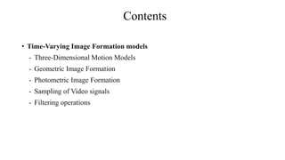
This document discusses the basic steps involved in video processing, including:
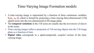
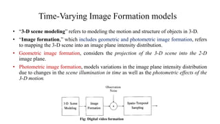
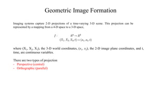
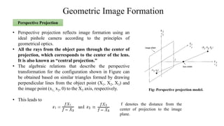
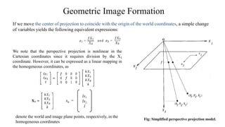
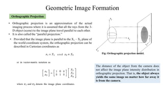
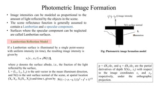
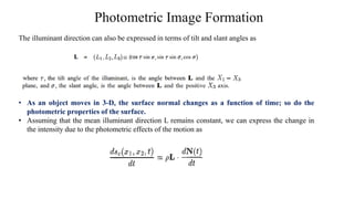
1) Time-varying image formation models which describe how a 3D scene is projected into a 2D image plane over time. This includes modeling 3D motion and structure, as well as geometric and photometric image formation.
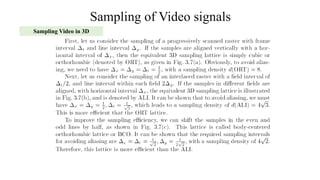
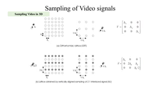
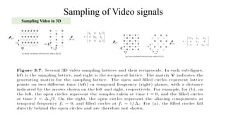
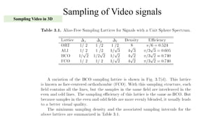
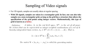
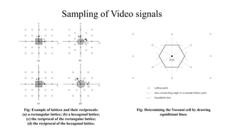
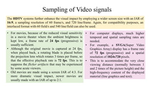
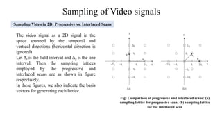
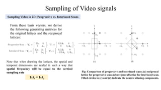
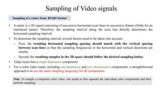
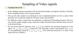
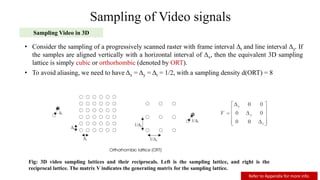
2) Sampling of video signals which involves converting continuous video signals to discrete digital signals using sampling and quantization. Key aspects like sampling rates, progressive vs interlaced scanning are covered.
3) Filtering operations which are mathematical operations used to process video signals like removing noise or extracting information.

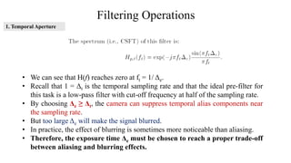
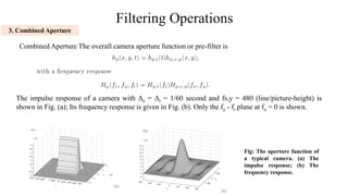
![Filtering Operations
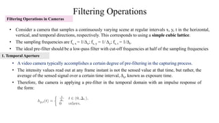
• In addition to temporal integration, the camera also performs spatial integration.
• The value read-out at any pixel (a position on a scan line with a tube-based camera or a sensor
in a CCD [Charge Coupled Device] camera) is not the optical signal at that point alone, rather a
weighted integration of the signals in a small window surrounding it, called aperture.
• The shape of the aperture and the weighting values constitute the camera spatial aperture function.
This aperture function serves as the spatial pre-filter, and its Fourier transform is known as the
modulation transfer function (MTF) of the camera.
• With most cameras, the spatial aperture function can be approximated by a circularly symmetric
Gaussian function
2. Spatial Aperture](https://image.slidesharecdn.com/basicstepsofvideoprocessing-unit42-230108125047-4a8e7d96/85/Basic-Steps-of-Video-Processing-unit-4-2-pdf-35-320.jpg)