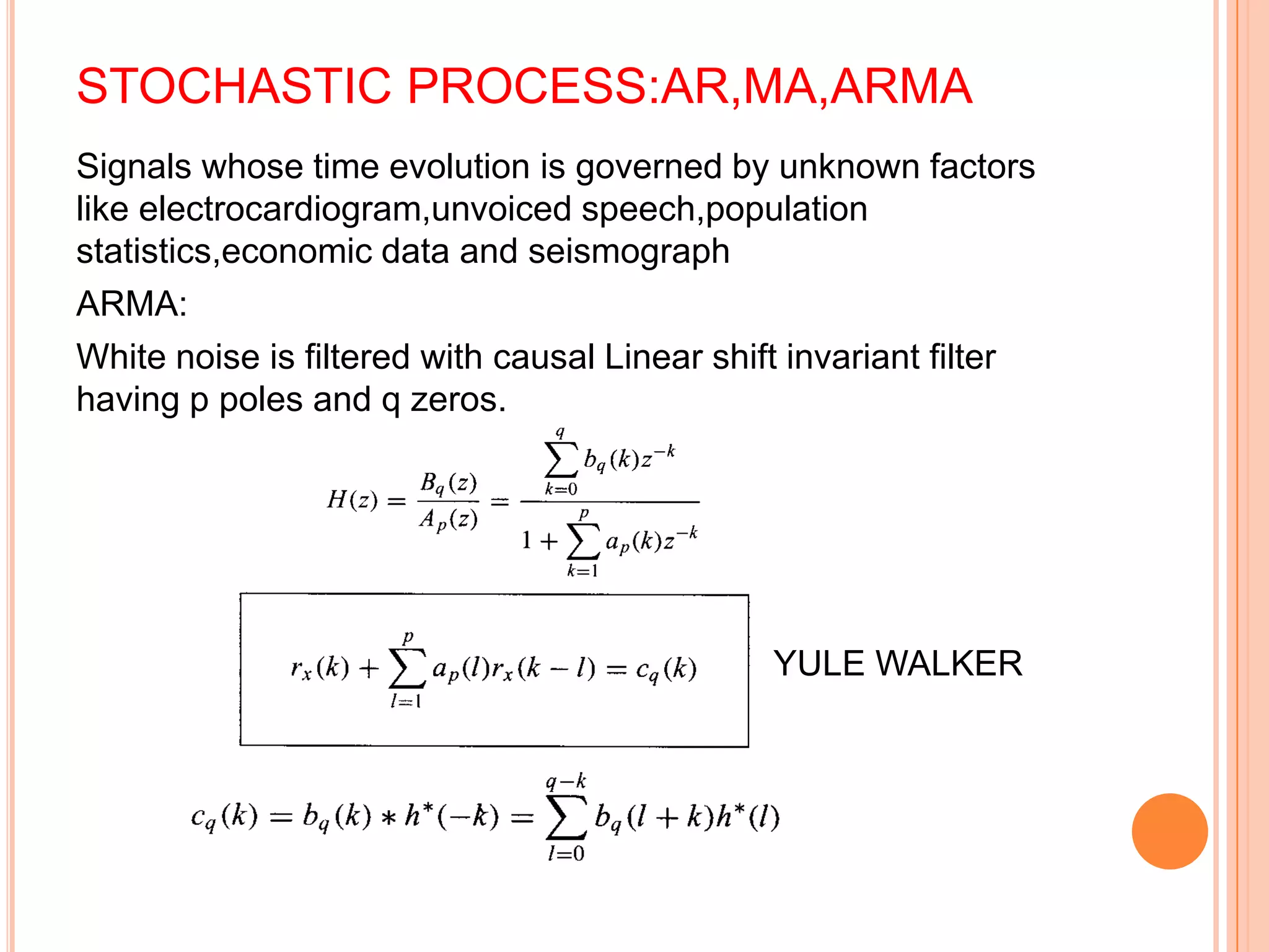
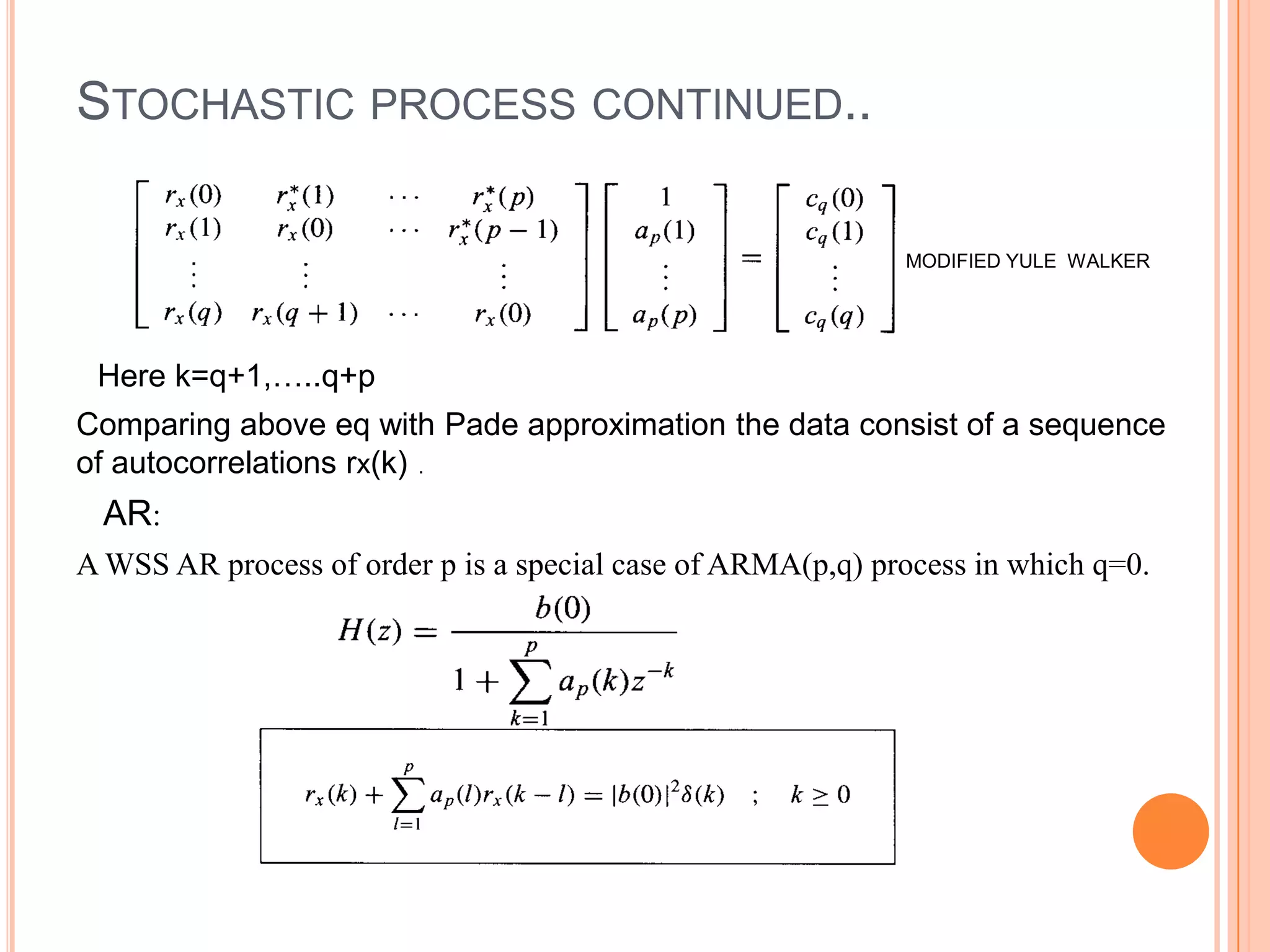
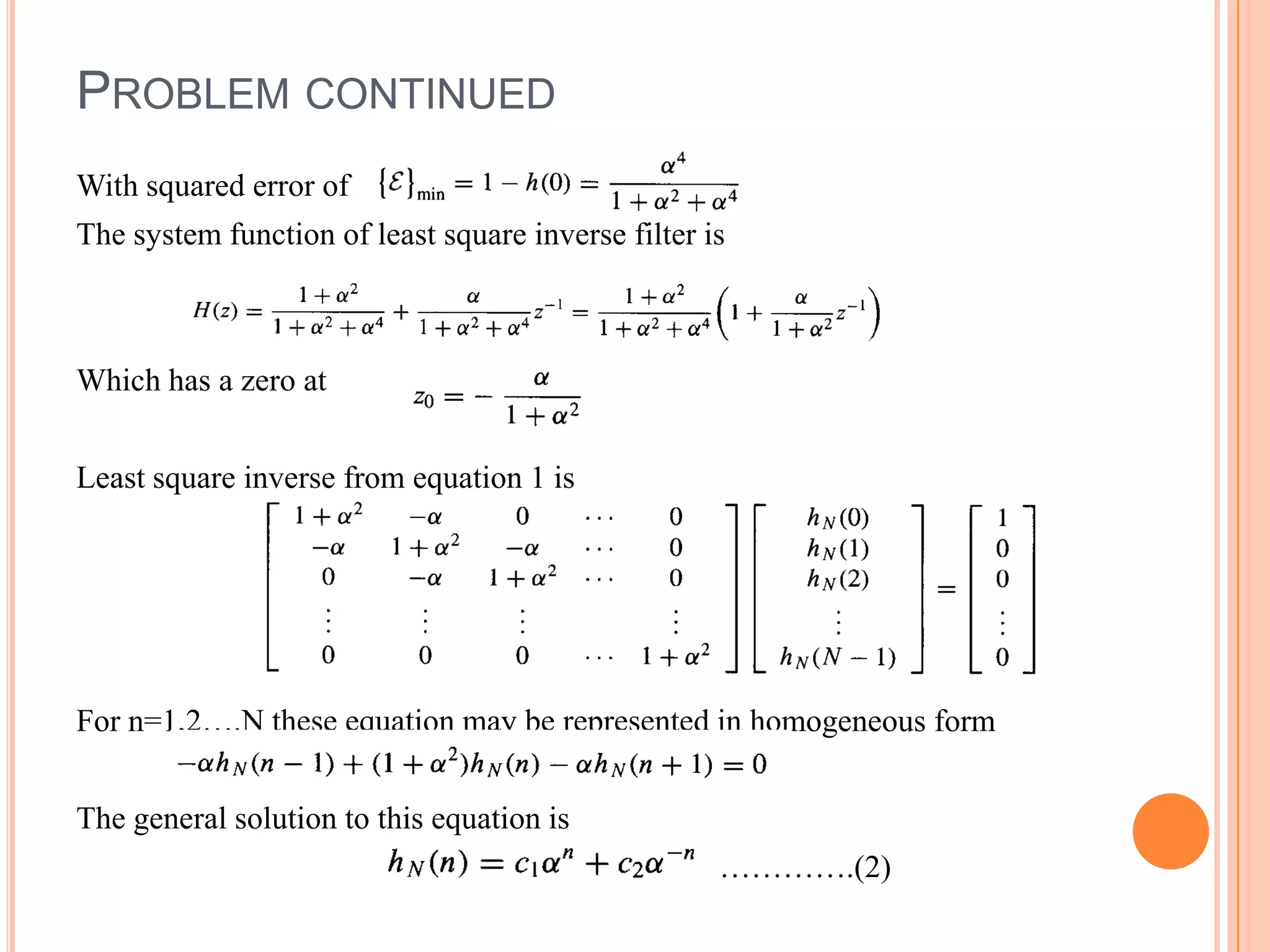
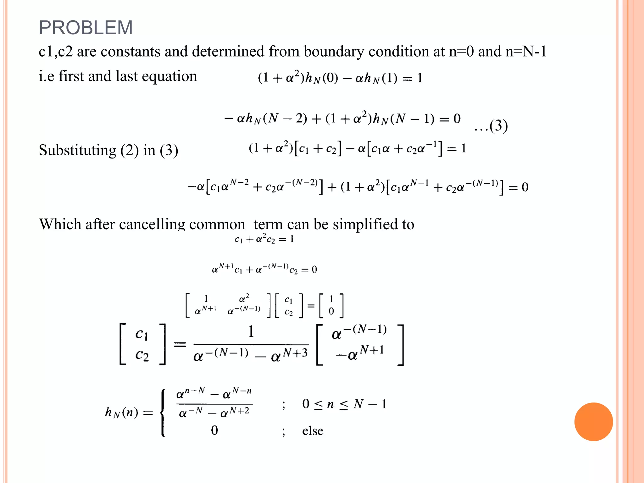
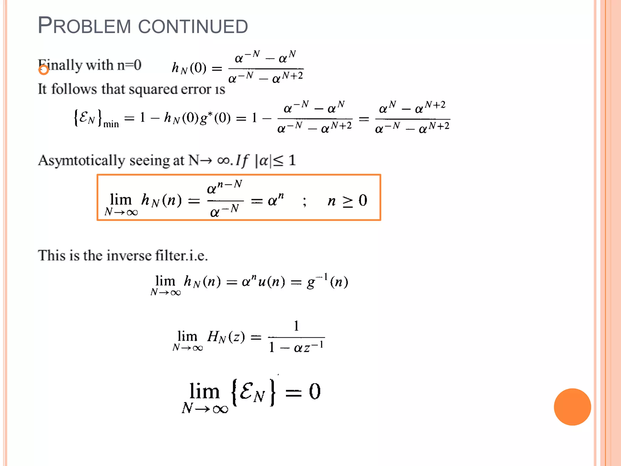
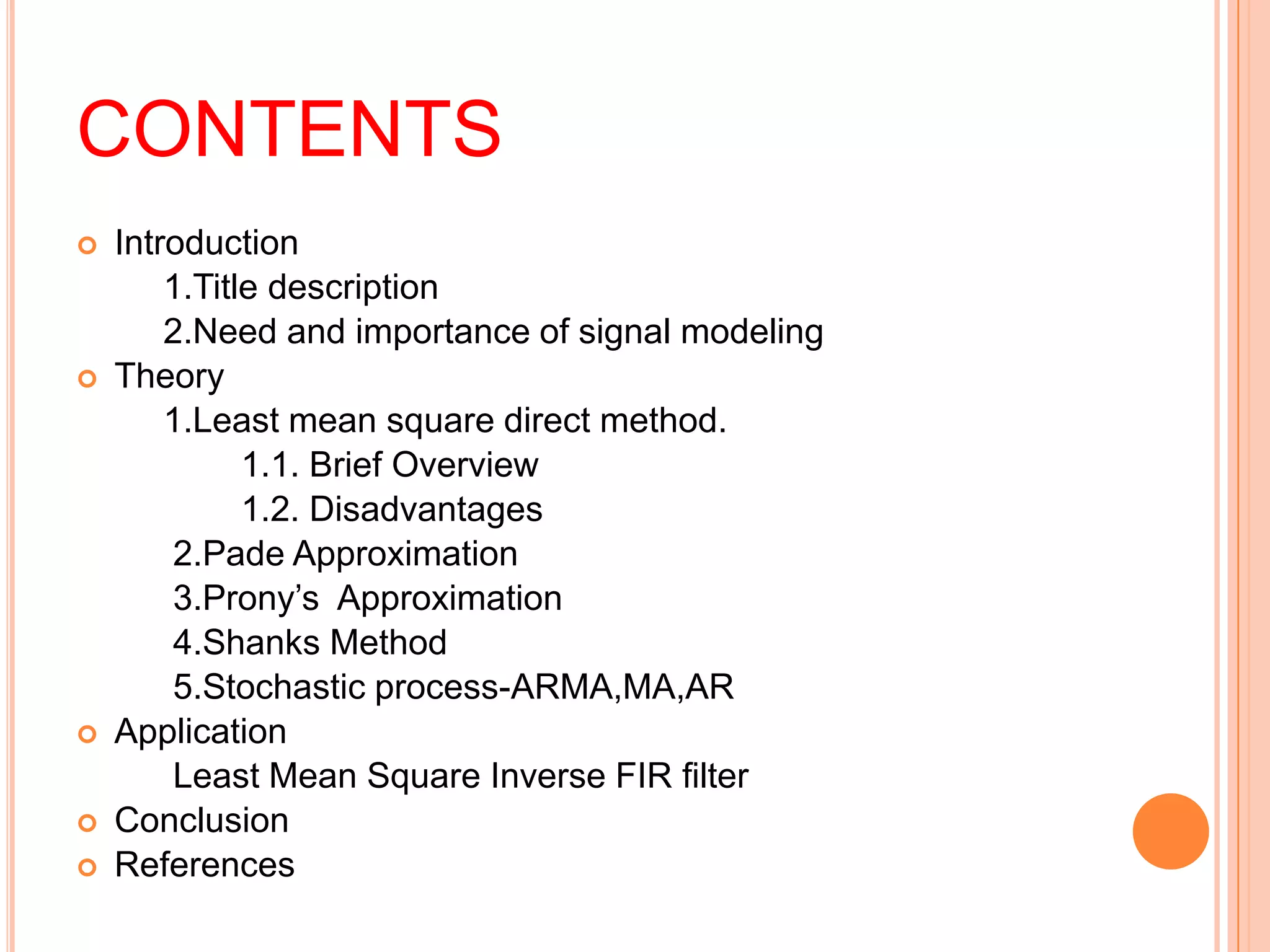
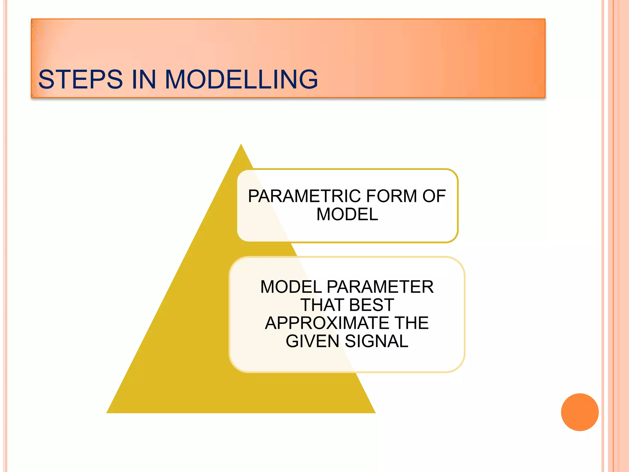
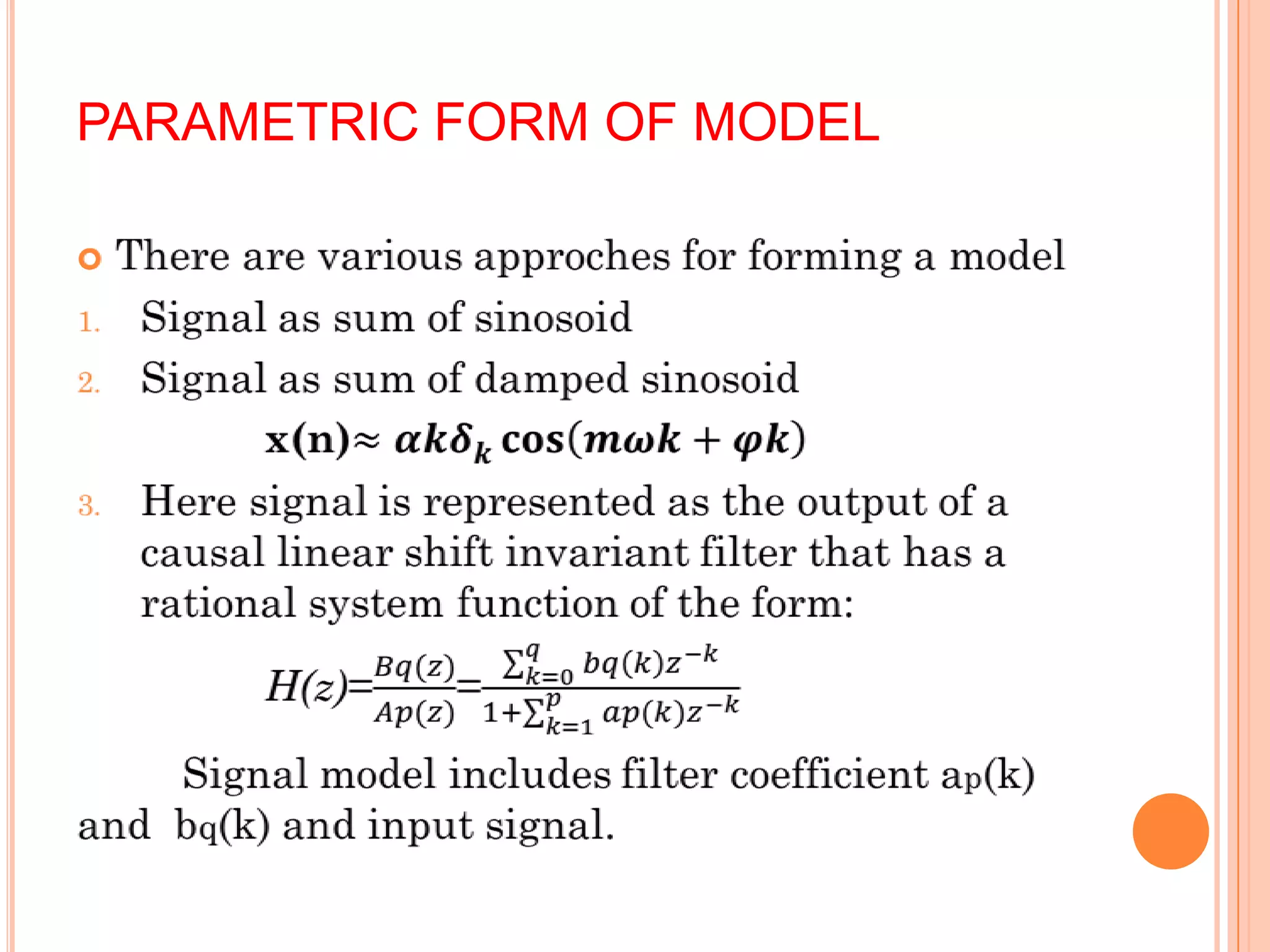
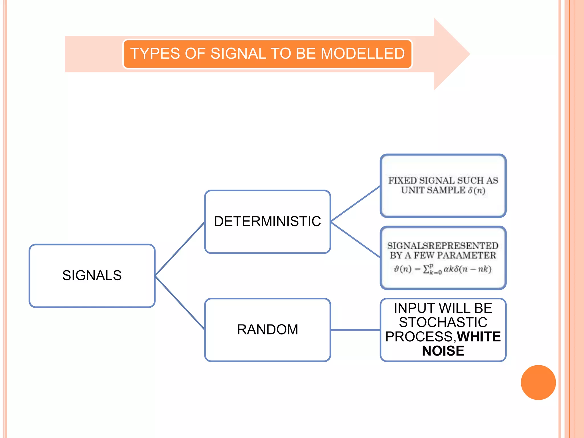
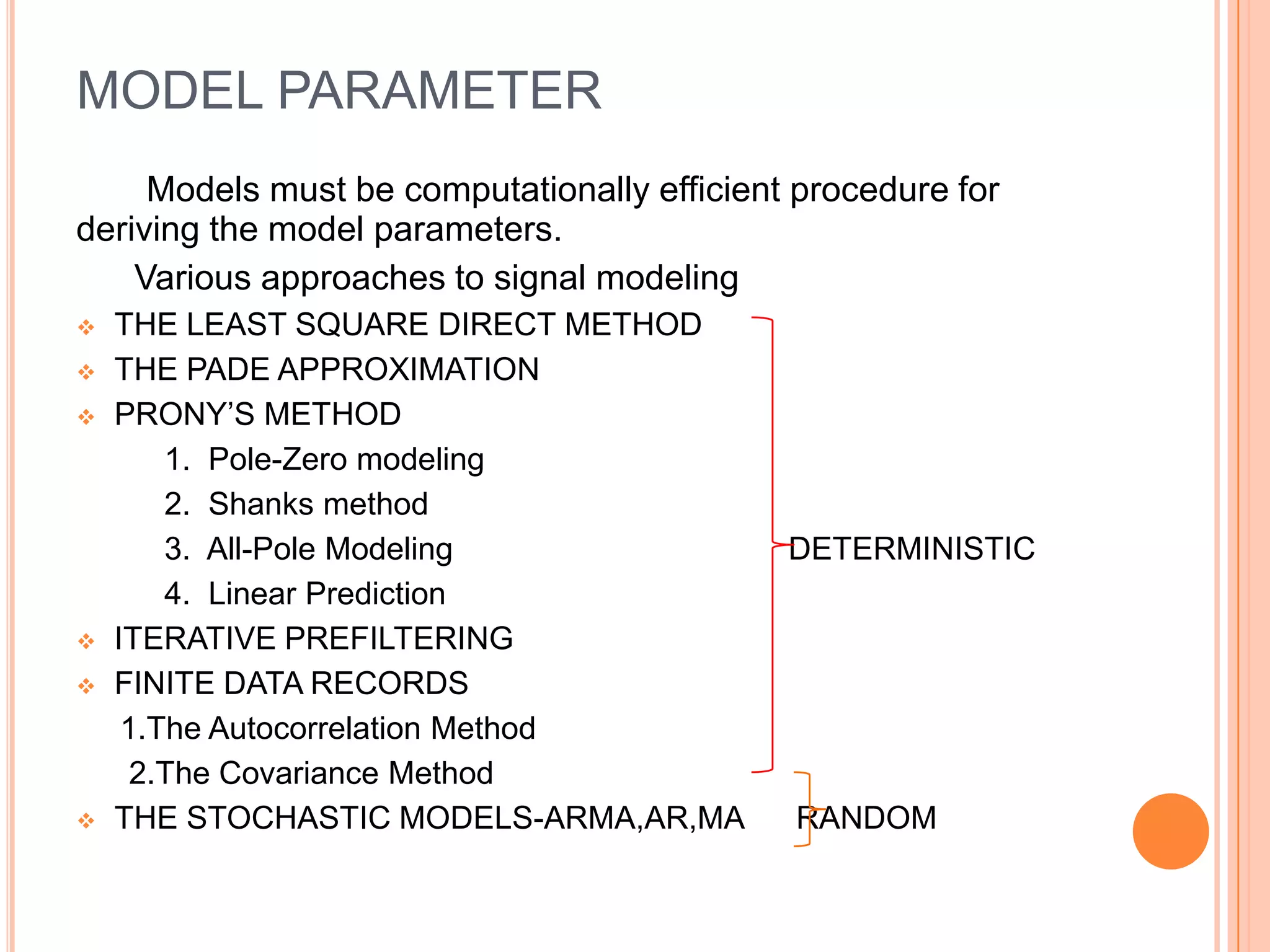
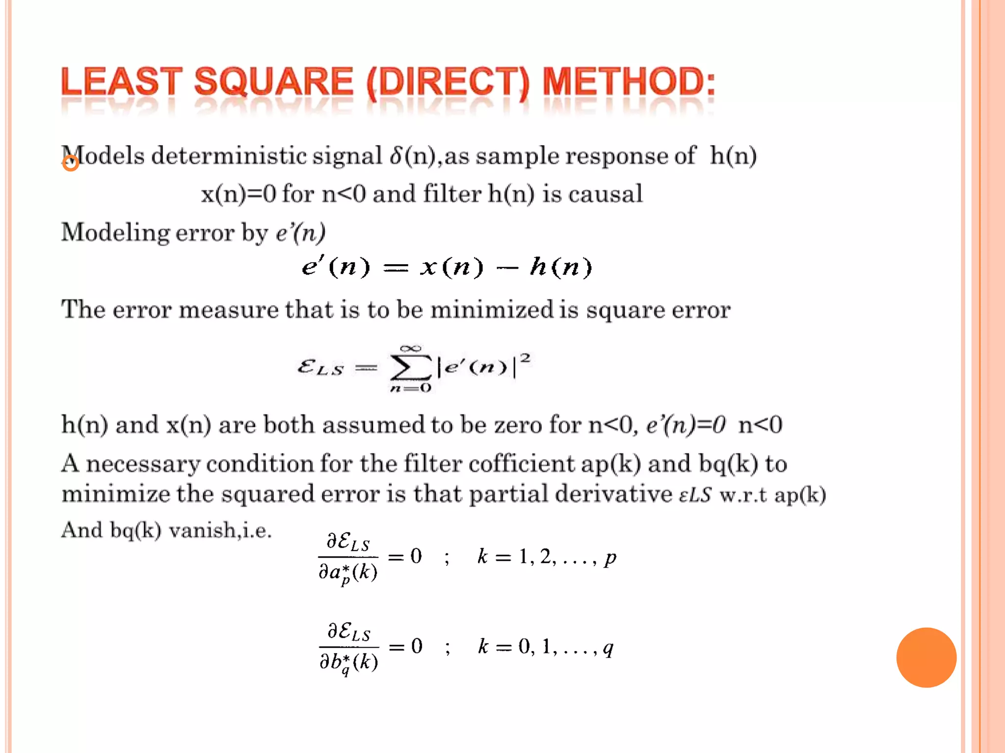
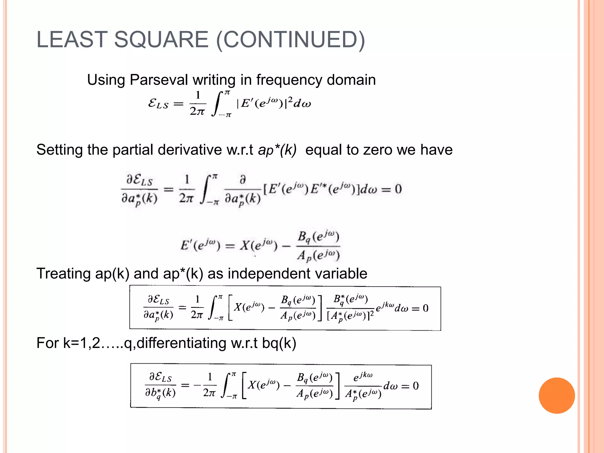
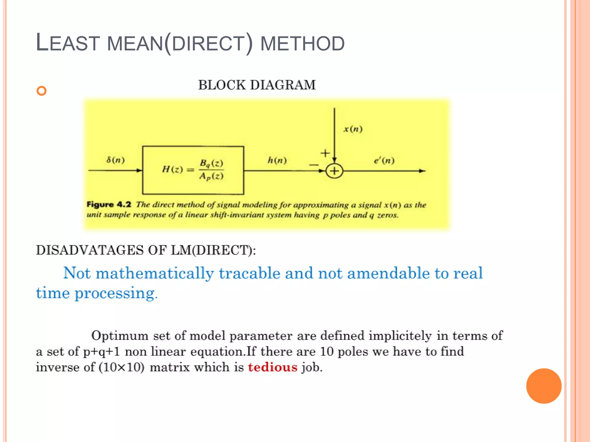
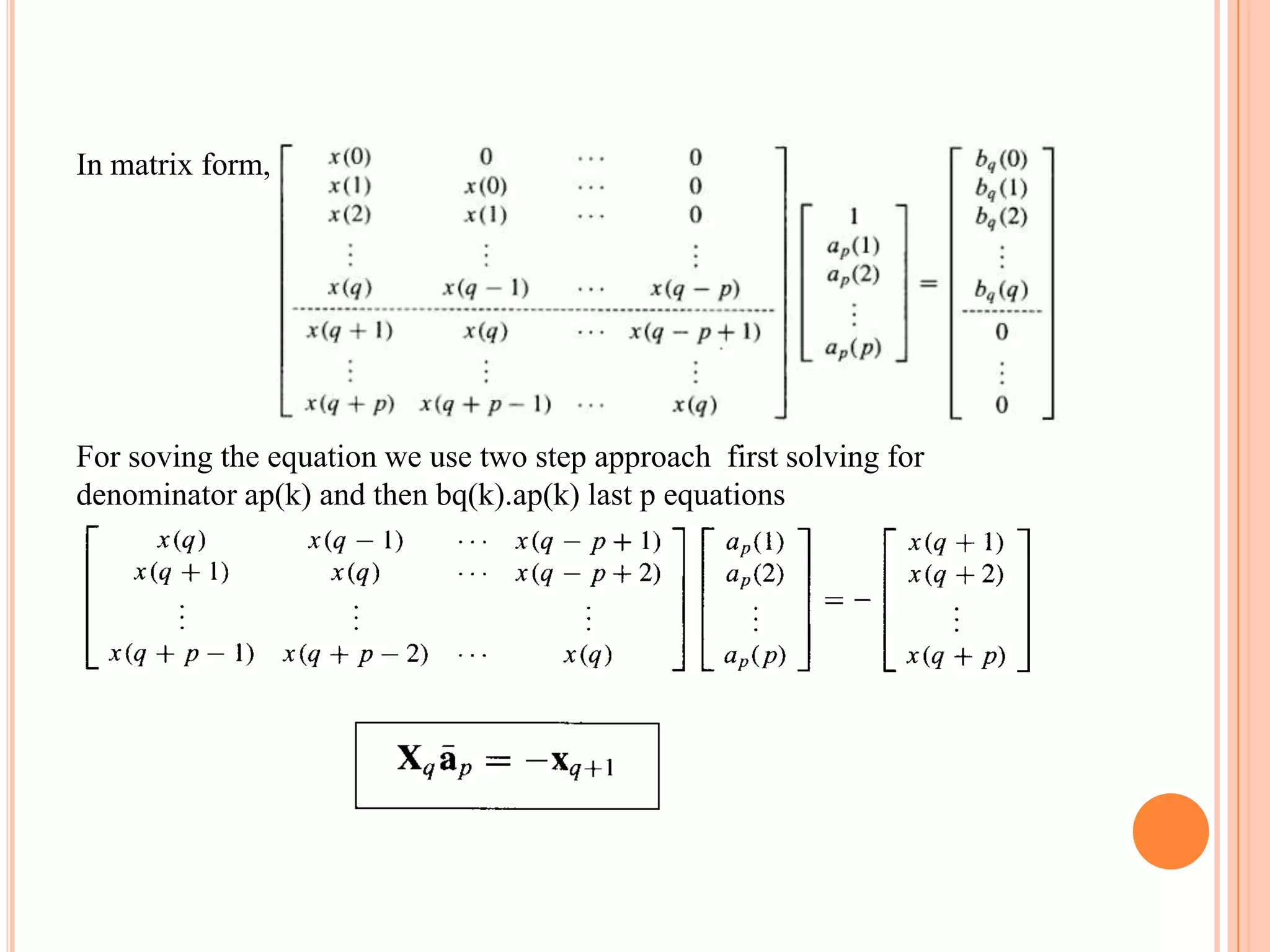
This document discusses various methods for modeling signals, including deterministic and stochastic processes. It covers topics like the least mean square direct method, Pade approximation, Prony's method, Shanks method, and stochastic processes like ARMA, MA, and AR. It also discusses an application of signal modeling for designing a least squares inverse FIR filter. Model order estimation is noted as an important problem in signal modeling when the correct model order is unknown.

1. SIGNAL MODELING
BY
DEBANGI GOSWAMI

2. CONTENTS
 Introduction
1.Title description
2.Need and importance of signal modeling
 Theory
1.Least mean square direct method.
1.1. Brief Overview
1.2. Disadvantages
2.Pade Approximation
3.Prony’s Approximation
4.Shanks Method
5.Stochastic process-ARMA,MA,AR
 Application
Least Mean Square Inverse FIR filter
 Conclusion
 References

3. WHAT IS MODELING:
 Modelling of signal is basically mathematical
representation of signal.
 Fourier series, Fourier transform are kind of signal
models.
WHY MODELLING
NEED OF MODELING:
1.EFFICIENCY OF TRANSMISSION
2.PREDICTION

4. SIGNAL MODELING IN EFFICIENCY OF
TRANSMISSION


5. SIGNAL MODELING IN
PREDICTION


6. STEPS IN MODELLING
PARAMETRIC FORM OF
MODEL
MODEL PARAMETER
THAT BEST
APPROXIMATE THE
GIVEN SIGNAL

7. PARAMETRIC FORM OF MODEL


8. TYPES OF SIGNAL TO BE MODELLED
DETERMINISTIC
SIGNALS
INPUT WILL BE
STOCHASTIC
RANDOM
PROCESS,WHITE
NOISE

9. MODEL PARAMETER
Models must be computationally efficient procedure for
deriving the model parameters.
Various approaches to signal modeling
 THE LEAST SQUARE DIRECT METHOD
 THE PADE APPROXIMATION
 PRONY’S METHOD
1. Pole-Zero modeling
2. Shanks method
3. All-Pole Modeling DETERMINISTIC
4. Linear Prediction
 ITERATIVE PREFILTERING
 FINITE DATA RECORDS
1.The Autocorrelation Method
2.The Covariance Method
 THE STOCHASTIC MODELS-ARMA,AR,MA RANDOM

10. 

11. LEAST SQUARE (CONTINUED)
Using Parseval writing in frequency domain
Setting the partial derivative w.r.t ap*(k) equal to zero we have
Treating ap(k) and ap*(k) as independent variable
For k=1,2…..q,differentiating w.r.t bq(k)

12. LEAST MEAN(DIRECT) METHOD


13. PADE APPROXIMATION
 Pade approximation only requires solving a set linear equation.
 In Pade we force the filter output h(n) to be equal to given signal x(n)
for p+q+1 values of n.
In time domain,
Where h(n)=0 for n<0 and n>q.To find the cofficients ap(k) and bq(k)
that gives an exact fit of data model in [0,p+q] we set h(n)=x(n)

14. In matrix form,
For soving the equation we use two step approach first solving for
denominator ap(k) and then bq(k).ap(k) last p equations

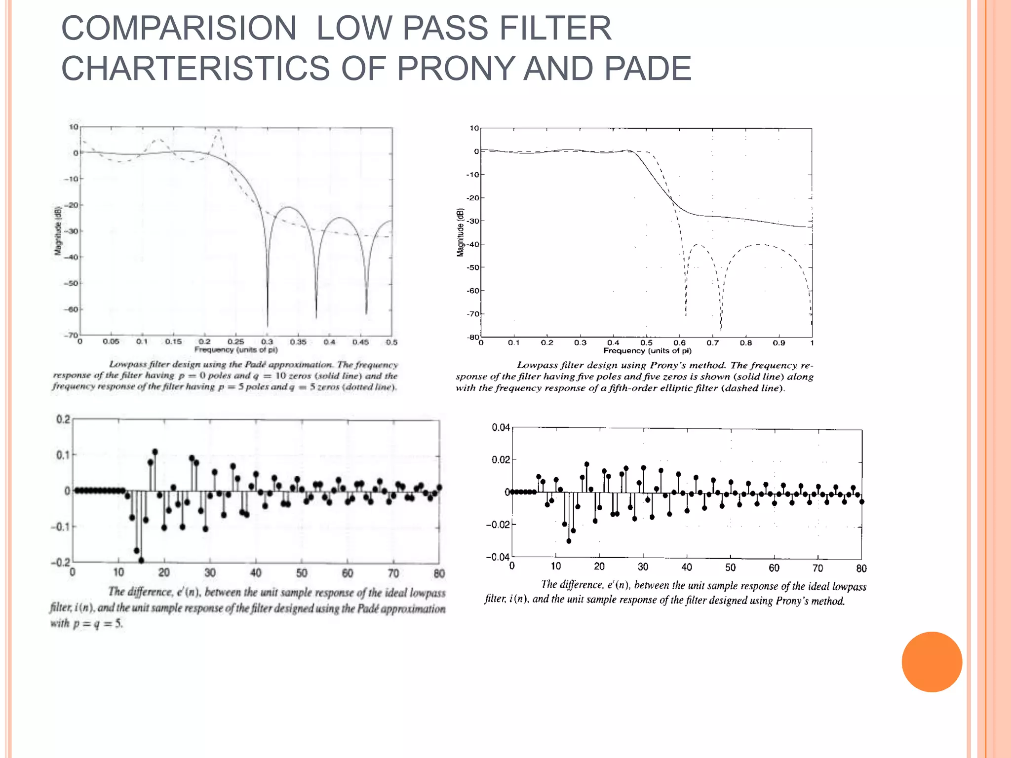
15. CONCLUSIONS ON PADE APPROXIMATION
 The model formed from Pade approximation will
produce an exact fit to data over the
interval[0,p+q].But has no guarantee on how
accurate the model will be for n>p+q.
 Pade approximation will give correct model
parameters provided the model order is chosen to
be large enough.
 Since the Pade approximation forces the model to
match the signal only over limited range of
values,the model generated is not stable

16. PRONY’S METHOD
The limitation of Pade approximation-Only uses values of the
signal x(n) over the interval [0,p+q] to determine model
parameter and over this interval, it models the signal without
error.
There is no guarantee on how well the model will
approximate the signal for n>p+q
POLE ZERO MODELLING:
Similar to pade x(n)=0 for n<0.A least square minimization of e’(n)
results in set of non-linear equation for filter cofficient
Multiplying by Ap(z) we have new error
That is linear cofficients.In time domain:

17. Since bq(n)=0 for n>q,error can be explicitly written as
Instead of setting e(n)=0 for n=0,1,…….p+q as in Pade
approximation,Prony’s method begins by finding the cofficient
ap(k) that minimizes squared error.

18. Equivalently,
Prony’s normal equation:
In matrix form normal equation are
Consisely written as

19. ESTIMATION OF ERROR IN PRONY’S
Minimun value of modeling error:
e(n) and x*(n) are uncorrelated so from orthogonality principle
the second term is zero.
Thus the minimum value:

20. PRONY NORMAL EQUATION
Augmenting the previous equation in this
Using matrix notation written as

21. COMPARISION LOW PASS FILTER
CHARTERISTICS OF PRONY AND PADE

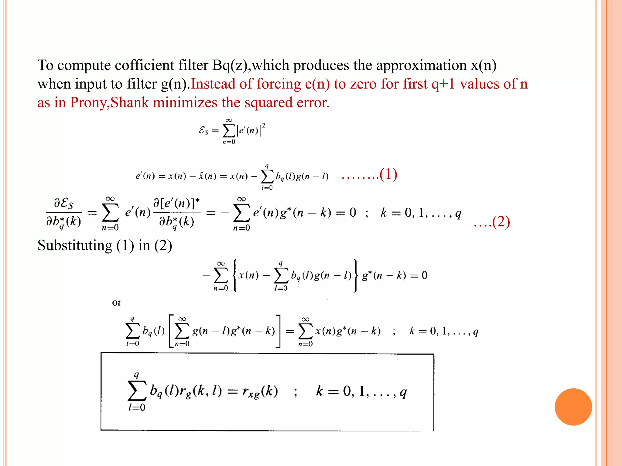
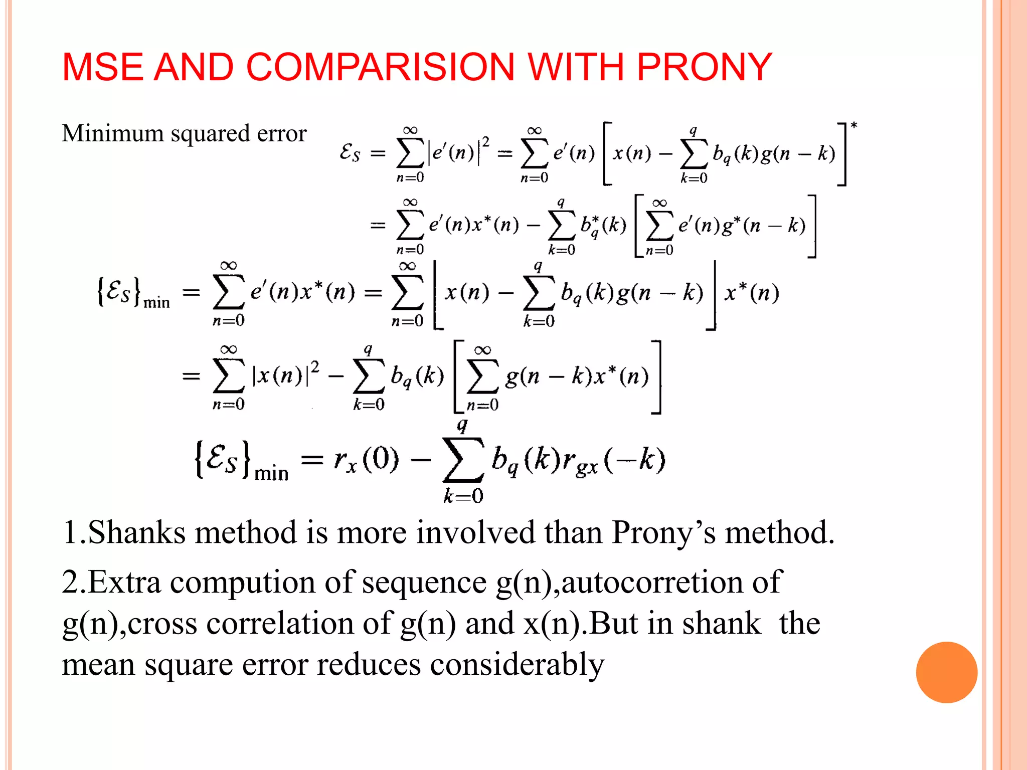
22. SHANKS APPROXIMATION
In Prony e(n)=0 for n=1, 2,….q.Although this allows the model to be exact
over [0,q],this does not take into account data for n>q.
Shanks performs mininization of model error over entire length of data record.
Filter can be viewed as cascade of two filter Ap(z) and Bq(z)
g(n) can be computed using the equation:

23. To compute cofficient filter Bq(z),which produces the approximation x(n)
when input to filter g(n).Instead of forcing e(n) to zero for first q+1 values of n
as in Prony,Shank minimizes the squared error.
……..(1)
………….(2)
Substituting (1) in (2)

24. MSE AND COMPARISION WITH PRONY
Minimum squared error
1.Shanks method is more involved than Prony’s method.
2.Extra compution of sequence g(n),autocorretion of
g(n),cross correlation of g(n) and x(n).But in shank the
mean square error reduces considerably

25. STOCHASTIC PROCESS:AR,MA,ARMA
Signals whose time evolution is governed by unknown factors
like electrocardiogram,unvoiced speech,population
statistics,economic data and seismograph
ARMA:
White noise is filtered with causal Linear shift invariant filter
having p poles and q zeros.
YULE WALKER

26. STOCHASTIC PROCESS CONTINUED..
MODIFIED YULE WALKER
Here k=q+1,…..q+p
Comparing above eq with Pade approximation the data consist of a sequence
of autocorrelations rx(k) .
AR:
A WSS AR process of order p is a special case of ARMA(p,q) process in which q=0.

27. STOCHASTIC CONTINUED….
In matrix form
MA: A MA process is generated by filtering unit variance white noise
with an FIR filter order q
:

28. APPLICATION OF SIGNAL MODELLING
FIR LEAST SQUARES INVERSE FILTER
Given a FIR filter the inverse filter relation can be written as
NEED:
 Equalization filter in digital communicatilon.Assume that channeal
transfer function is G(z),the eqalization filter is found by relation.
Procedure:
g(n) is causal filter to be equalized,the problem is to find FIR filter
hN(n) of length N such that
The equation is same as shank,the solution of least square inverse filter
is

29. FIR LS INVERSE FILTER CONTINUED
where
Matrix form:
From shank’s it follows the concise form: …………..(1)

30. PROBLEM ON LEAST SQUARE
INVERSE FIR FILTER


31. PROBLEM CONTINUED
With squared error of
The system function of least square inverse filter is
Which has a zero at
Least square inverse from equation 1 is
For n=1,2….N these equation may be represented in homogeneous form
The general solution to this equation is
………….(2)

32. PROBLEM
c1,c2 are constants and determined from boundary condition at n=0 and n=N-1
i.e first and last equation
…(3)
Substituting (2) in (3)
Which after cancelling common term can be simplified to

33. PROBLEM CONTINUED


34. CONCLUSION
 The various methods of signal modelling for both
deterministic and stochastic process are discussed.
 PROBLEM IN SIGNAL MODELING
MODEL ORDER ESTIMATION:
In the cases assumed so far we have assumed that a model of given
order to be found.In the absence of any information about the correct
model order ,it becomes necessary to estimate what an appropiate
model order should be.Misleading information may result in an
inappropiate model order.

35. REFERENCES
 STATISTICAL SIGNAL PROCESSING AND MODELING…
MONSON H.HAYES
 Signal Modeling Techniques In Speech Recognition
by,Joseph Picone
 Spectrum Estimation and Modeling by Petar M. Djuri´c State
University of New York at Stony Brook Steven M. Kay
University of Rhode Island
 SOME REMARKS ON PADÉ-APPROXIMATIONS M.Vajta
 Comparing Autoregressive Moving Average(ARMA)
coefficients determination using Artificial Neural Networks with
other techniques Abiodun M. Aibinu, Momoh J. E. Salami,
Amir A. Shafie and Athaur Rahman Najeeb

36. THANKS FOR YOUR ATTENTION