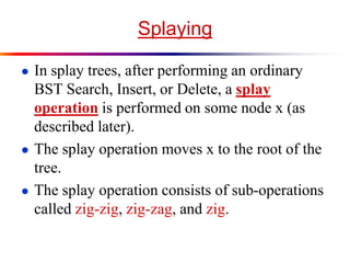
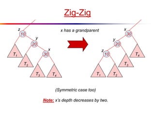
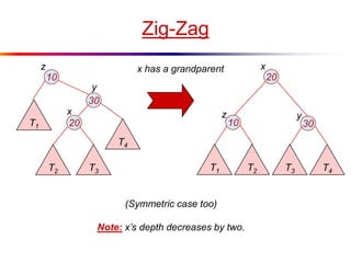
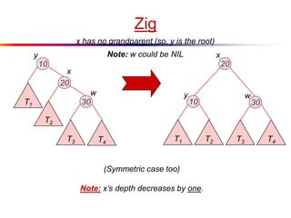
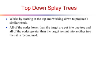
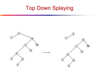
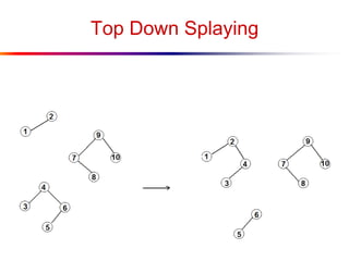
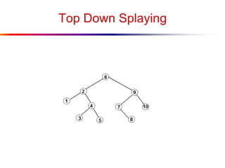
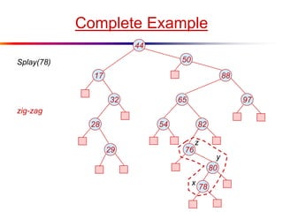
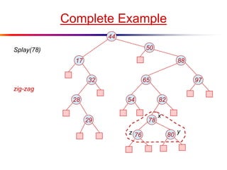
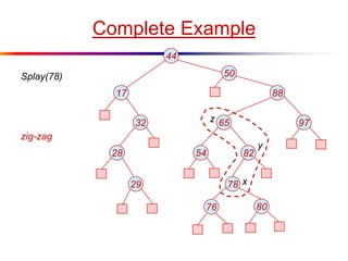
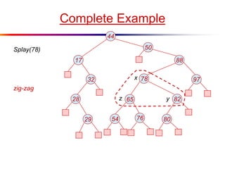
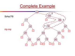
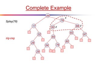
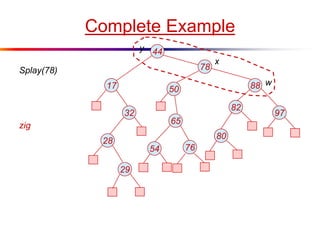
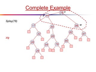
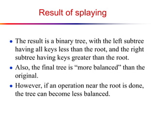
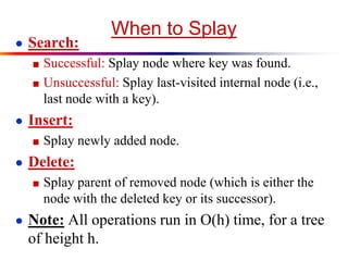
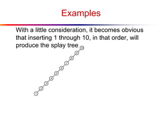
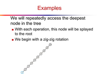
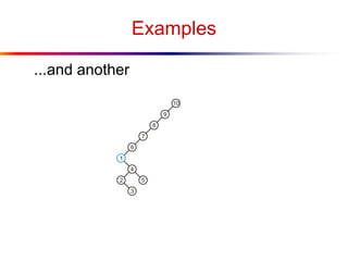
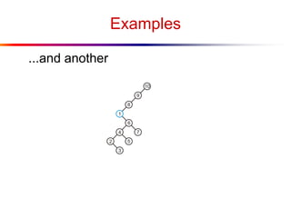
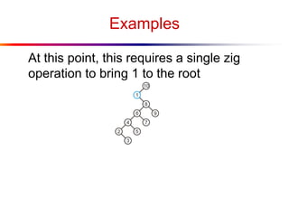
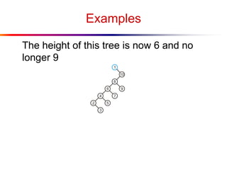
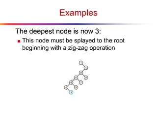
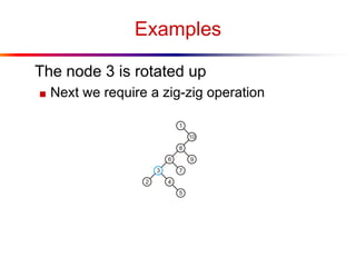
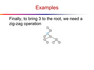
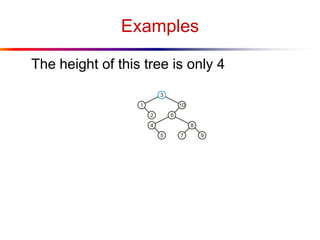
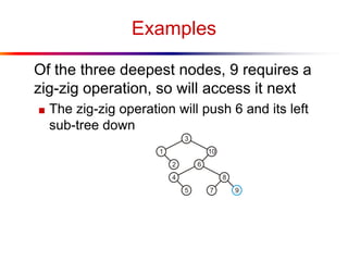
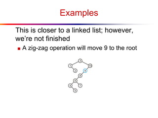
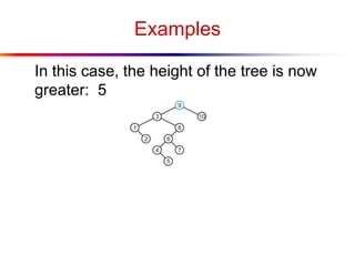
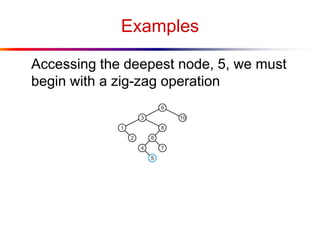
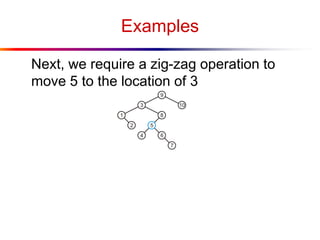
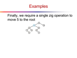
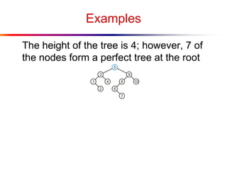
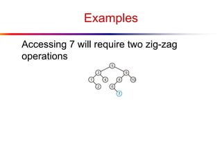
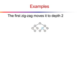
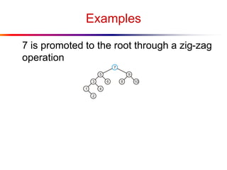
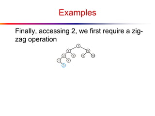
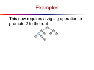
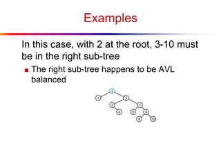
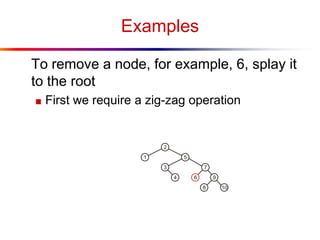
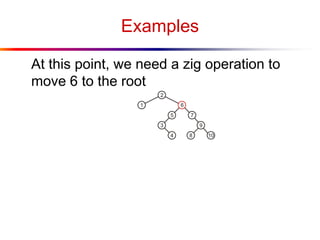
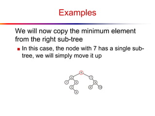
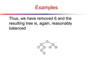
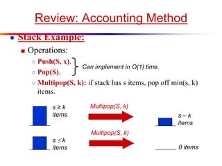
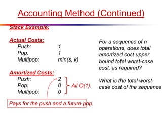
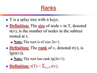
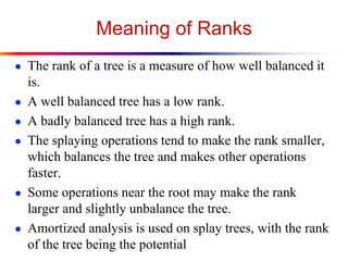
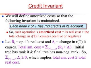
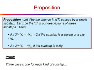
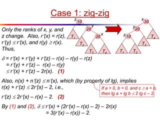
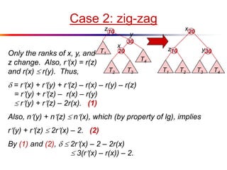
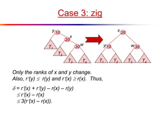
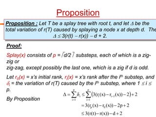
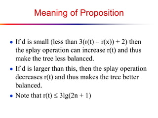
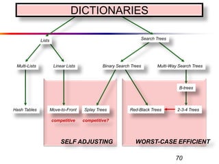
The document describes splay trees, a type of self-adjusting binary search tree. Splay trees differ from other balanced binary search trees in that they do not explicitly rebalance after each insertion or deletion, but instead perform a process called "splaying" in which nodes are rotated to the root. This splaying process helps ensure search, insert, and delete operations take O(log n) amortized time. The document explains splaying operations like zig, zig-zig, and zig-zag that rotate nodes up the tree, and analyzes how these operations affect the tree's balance over time through a concept called the "rank" of the tree.

1. Algorithms
Splay Trees

2. Splay Trees
● In balanced tree schemes, explicit rules are
followed to ensure balance.
● In splay trees, there are no such rules.
● Search, insert, and delete operations are like in
binary search trees, except at the end of each
operation a special step called splaying is done.
● Splaying ensures that all operations take O(lg n)
amortized time.
● First, a quick review of BST operations…

3. BST: Search
44
8817
65 9732
28 54 82
7629
80
Note: In the handout,
sentinel leaf nodes are
assumed.
 tree with n keys
has 2n+1 nodes.
Search(25) Search(76)

4. BST: Insert
44
8817
65 9732
28 54 82
7629
80
Insert(78)
78

5. BST: Delete
44
8817
65 9732
28 54 82
7629
80
78
Delete(32)
Has only one
child: just splice
out 32.

6. BST: Delete
44
8817
65 9728
54 82
76
29
80
78
Delete(32)

7. BST: Delete
44
8817
65 9732
28 54 82
7629
80
78
Delete(65)
Has two children:
Replace 65 by successor,
76, and splice out
successor.
Note: Successor can have
at most one child. (Why?)

8. BST: Delete
44
8817
76 9732
28 54 82
29 80
78
Delete(65)

9. Splaying
● In splay trees, after performing an ordinary
BST Search, Insert, or Delete, a splay
operation is performed on some node x (as
described later).
● The splay operation moves x to the root of the
tree.
● The splay operation consists of sub-operations
called zig-zig, zig-zag, and zig.

10. Zig-Zig
10
20
30
T3 T4
T2
T1
z
y
x
30
20
10
T1 T2
T3
T4
x
y
z
(Symmetric case too)
Note: x’s depth decreases by two.
x has a grandparent

11. Zig-Zag
10
30
20
T3
T4
T2
T1
z
y
x
20
10
T1 T2 T3 T4
x
z
(Symmetric case too)
Note: x’s depth decreases by two.
30
y
x has a grandparent

12. Zig
20
10
T1 T2 T3 T4
x
y
(Symmetric case too)
Note: x’s depth decreases by one.
30
w
10
20
30
T3 T4
T2
T1
y
x
w
x has no grandparent (so, y is the root)
Note: w could be NIL

13. Top Down Splay Trees
● Works by starting at the top and working down to produce a
similar result.
● All of the nodes lower than the target are put into one tree and
all of the nodes greater than the target are put into another tree
then it is recombined.

14. Top Down Splaying

15. Top Down Splaying

16. Top Down Splaying

17. Complete Example
44
8817
65 9732
28 54 82
7629
80
78
Splay(78) 50
x
y
z
zig-zag

18. Complete Example
44
8817
65 9732
28 54 82
7829
8076
Splay(78) 50
zig-zag
x
yz

19. Complete Example
44
8817
65 9732
28 54 82
7829
8076
Splay(78) 50
x
y
z
zig-zag

20. Complete Example
44
8817
65
9732
28
54
82
78
29 8076
Splay(78) 50
zig-zag
z y
x

21. Complete Example
44
8817
65
9732
28
54
82
78
29 8076
Splay(78) 50
x
y
z
zig-zag

22. Complete Example
44
8817
65
9732
28
54
82
29
80
76
Splay(78)
50
78
zig-zag
z
y
x

23. Complete Example
44
8817
65
9732
28
54
82
29
80
76
Splay(78)
50
78
y
x
w
zig

24. Complete Example
44
8817
65
9732
28
54
82
29
80
76
Splay(78)
50
78 x
y
w
zig

25. Result of splaying
● The result is a binary tree, with the left subtree
having all keys less than the root, and the right
subtree having keys greater than the root.
● Also, the final tree is “more balanced” than the
original.
● However, if an operation near the root is done,
the tree can become less balanced.

26. When to Splay
● Search:
■ Successful: Splay node where key was found.
■ Unsuccessful: Splay last-visited internal node (i.e.,
last node with a key).
● Insert:
■ Splay newly added node.
● Delete:
■ Splay parent of removed node (which is either the
node with the deleted key or its successor).
● Note: All operations run in O(h) time, for a tree
of height h.

27. Examples
With a little consideration, it becomes obvious
that inserting 1 through 10, in that order, will
produce the splay tree

28. Examples
We will repeatedly access the deepest
node in the tree
■ With each operation, this node will be splayed
to the root
■ We begin with a zig-zig rotation

29. Examples
This is followed by another zig-zig
operation...

30. Examples
...and another

31. Examples
...and another

32. Examples
At this point, this requires a single zig
operation to bring 1 to the root

33. Examples
The height of this tree is now 6 and no
longer 9

34. Examples
The deepest node is now 3:
■ This node must be splayed to the root
beginning with a zig-zag operation

35. Examples
The node 3 is rotated up
■ Next we require a zig-zig operation

36. Examples
Finally, to bring 3 to the root, we need a
zig-zag operation

37. Examples
The height of this tree is only 4

38. Examples
Of the three deepest nodes, 9 requires a
zig-zig operation, so will access it next
■ The zig-zig operation will push 6 and its left
sub-tree down

39. Examples
This is closer to a linked list; however,
we’re not finished
■ A zig-zag operation will move 9 to the root

40. Examples
In this case, the height of the tree is now
greater: 5

41. Examples
Accessing the deepest node, 5, we must
begin with a zig-zag operation

42. Examples
Next, we require a zig-zag operation to
move 5 to the location of 3

43. Examples
Finally, we require a single zig operation to
move 5 to the root

44. Examples
The height of the tree is 4; however, 7 of
the nodes form a perfect tree at the root

45. Examples
Accessing 7 will require two zig-zag
operations

46. Examples
The first zig-zag moves it to depth 2

47. Examples
7 is promoted to the root through a zig-zag
operation

48. Examples
Finally, accessing 2, we first require a zig-
zag operation

49. Examples
This now requires a zig-zig operation to
promote 2 to the root

50. Examples
In this case, with 2 at the root, 3-10 must
be in the right sub-tree
■ The right sub-tree happens to be AVL
balanced

51. Examples
To remove a node, for example, 6, splay it
to the root
■ First we require a zig-zag operation

52. Examples
At this point, we need a zig operation to
move 6 to the root

53. Examples
We will now copy the minimum element
from the right sub-tree
■ In this case, the node with 7 has a single sub-
tree, we will simply move it up

54. Examples
Thus, we have removed 6 and the
resulting tree is, again, reasonably
balanced

55. Amortized Analysis
● Based on the Accounting Method
■ Idea: When an operation’s amortized cost exceeds
it actual cost, the difference is assigned to certain
tree nodes as credit.
■ Credit is used to pay for subsequent operations
whose amortized cost is less than their actual cost.
● Most of our analysis will focus on splaying.
■ The BST operations will be easily dealt with at the
end.

56. Review: Accounting Method
● Stack Example:
■ Operations:
○ Push(S, x).
○ Pop(S).
○ Multipop(S, k): if stack has s items, pop off min(s, k)
items.
s ≥ k
items
s  k
items
Multipop(S, k)
Multipop(S, k)
s – k
items
0 items
Can implement in O(1) time.

57. Accounting Method (Continued)
● We charge each operation an amortized cost.
● Charge may be more or less than actual cost.
● If more, then we have credit.
● This credit can be used to pay for future
operations whose amortized cost is less than
their actual cost.
● Require: For any sequence of operations,
amortized cost upper bounds worst-case cost.
■ That is, we always have nonnegative credit.

58. Accounting Method (Continued)
Stack Example:
Actual Costs:
Push: 1
Pop: 1
Multipop: min(s, k)
Amortized Costs:
Push: 2
Pop: 0
Multipop: 0
Pays for the push and a future pop.
All O(1).
For a sequence of n
operations, does total
amortized cost upper
bound total worst-case
cost, as required?
What is the total worst-
case cost of the sequence?

59. Ranks
● T is a splay tree with n keys.
● Definition: The size of node v in T, denoted
n(v), is the number of nodes in the subtree
rooted at v.
■ Note: The root is of size 2n+1.
● Definition: The rank of v, denoted r(v), is
lg(n(v)).
■ Note: The root has rank lg(2n+1).
● Definition: r(T) = vT r(v).

60. Meaning of Ranks
● The rank of a tree is a measure of how well balanced it
is.
● A well balanced tree has a low rank.
● A badly balanced tree has a high rank.
● The splaying operations tend to make the rank smaller,
which balances the tree and makes other operations
faster.
● Some operations near the root may make the rank
larger and slightly unbalance the tree.
● Amortized analysis is used on splay trees, with the rank
of the tree being the potential

61. Credit Invariant
● We will define amortized costs so that the
following invariant is maintained.
■ So, each operation’s amortized cost = its real cost + the
total change in r(T) it causes (positive or negative).
● Let Ri = op. i’s real cost and i = change in r(T) it
causes. Total am. cost = i=1,…,n (Ri + i). Initial
tree has rank 0 & final tree has non-neg. rank. So,
i=1,…n i  0, which implies total am. cost  total
real cost.
Each node v of T has r(v) credits in its account.

62. What’s Left?
● We want to show that the per-operation amortized
cost is logarithmic.
● To do this, we need to look at how BST operations
and splay operations affect r(T).
■ We spend most of our time on splaying, and consider the
specific BST operations later.
● To analyze splaying, we first look at how r(T)
changes as a result of a single substep, i.e., zig, zig-
zig, or zig-zag.
■ Notation: Ranks before and after a substep are denoted
r(v) and r(v), respectively.

63. Proposition
Proposition : Let  be the change in r(T) caused by a single
substep. Let x be the “x” in our descriptions of these
substeps. Then,
•   3(r(x)  r(x))  2 if the substep is a zig-zig or a zig-
zag;
•   3(r(x)  r(x)) if the substep is a zig.
Proof:
Three cases, one for each kind of substep…

64. Case 1: zig-zig
10
20
30
T3 T4
T2
T1
z
y
x
30
20
10
T1 T2
T3
T4
x
y
z
Only the ranks of x, y, and
z change. Also, r(x) = r(z),
r(y)  r(x), and r(y)  r(x).
Thus,
 = r(x) + r(y) + r(z) – r(x) – r(y) – r(z)
= r(y) + r(z) – r(x) – r(y)
 r(x) + r(z) – 2r(x). (1)
Also, n(x) + n(z)  n(x), which (by property of lg), implies
r(x) + r(z)  2r(x) – 2, i.e.,
r(z)  2r(x) – r(x) – 2. (2)
By (1) and (2),   r(x) + (2r(x) – r(x) – 2) – 2r(x)
= 3(r(x) – r(x)) – 2.
If a > 0, b > 0, and c  a + b,
then lg a + lg b  2 lg c – 2.

65. Case 2: zig-zag
Only the ranks of x, y, and
z change. Also, r(x) = r(z)
and r(x)  r(y). Thus,
 = r(x) + r(y) + r(z) – r(x) – r(y) – r(z)
= r(y) + r(z) – r(x) – r(y)
 r(y) + r(z) – 2r(x). (1)
Also, n(y) + n(z)  n(x), which (by property of lg), implies
r(y) + r(z)  2r(x) – 2. (2)
By (1) and (2),   2r(x) – 2 – 2r(x)
 3(r(x) – r(x)) – 2.
10
30
20
T3
T4
T2
T1
z
y
x
20
10
T1 T2 T3 T4
x
z 30y

66. Case 3: zig
Only the ranks of x and y change.
Also, r(y)  r(y) and r(x)  r(x). Thus,
 = r(x) + r(y) – r(x) – r(y)
 r(x) – r(x)
 3(r(x) – r(x)).
20
10
T1 T2 T3 T4
x
y 30w
10
20
30
T3 T4
T2
T1
y
x
w

67. Proposition
Proposition : Let T be a splay tree with root t, and let  be the
total variation of r(T) caused by splaying a node x at depth d. The
  3(r(t)  r(x))  d + 2.
Proof:
Splay(x) consists of p = d/2 substeps, each of which is a zig-
zig or
zig-zag, except possibly the last one, which is a zig if d is odd.
Let r0(x) = x’s initial rank, ri(x) = x’s rank after the ith substep, and
i = the variation of r(T) caused by the ith substep, where 1  i 
p.
By Proposition
 
2dr(x))3(r(t)
22p(x))r(x)3(r
22(x))r(x)3(rδΔ
0p
p
1i
1ii
p
1i
i


  



68. Meaning of Proposition
● If d is small (less than 3(r(t)  r(x)) + 2) then
the splay operation can increase r(t) and thus
make the tree less balanced.
● If d is larger than this, then the splay operation
decreases r(t) and thus makes the tree better
balanced.
● Note that r(t)  3lg(2n + 1)

69. Comparisons
Advantages:
■ The amortized run times are similar to that of
AVL trees and red-black trees
■ The implementation is easier
■ No additional information (height/colour) is
required
Disadvantages:
■ The tree will change with read-only operations

70. Lists
Move-to-Front
Search Trees
Binary Search Trees Multi-Way Search Trees
B-trees
Splay Trees 2-3-4 TreesRed-Black Trees
SELF ADJUSTING WORST-CASE EFFICIENT
competitive competitive?
Linear ListsMulti-Lists
Hash Tables
DICTIONARIES
70