Downloaded 14 times


![MAX FLOW /MIN CUT ALGORITHM:
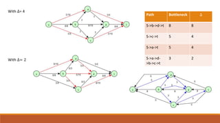
Let f` be the flow returned by our algorithm. Look at G` but define a cut in G.
Let (A`,B`) be the cut in G, where A`=[s,a] and B`= [ b,d,c,t].](https://image.slidesharecdn.com/networkflows-200912055505/85/Network-flows-15-320.jpg)
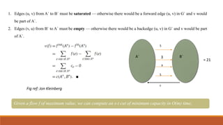


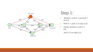


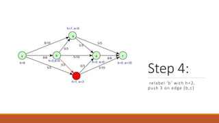


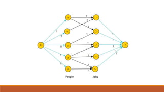


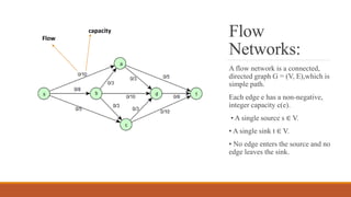
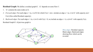
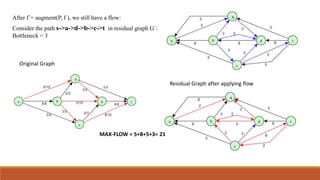
The document discusses network flows and algorithms for finding maximum flows in networks. It begins by defining a flow network as a directed graph with a source, sink, and edge capacities. The maximum flow problem is to find the maximum amount of flow that can be sent from the source to the sink respecting capacity constraints. The Ford-Fulkerson algorithm uses augmenting paths to iteratively increase the flow value. It runs in O(mC) time where m is edges and C is total capacity. The maximum flow value equals the minimum cut capacity, proven using residual graphs. Later sections discuss improvements like capacity scaling and preflow-push algorithms. Bipartite matching is also shown to reduce to a maximum flow problem.


![Ford_Fulkerson_Algorithm_uptade.ppt[1].pptx](https://cdn.slidesharecdn.com/ss_thumbnails/fordfulkersonalgorithmuptade-250128085250-50c85c74-thumbnail.jpg?width=640&height=640&fit=bounds)


