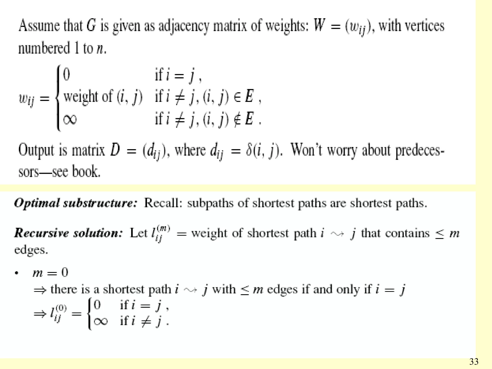
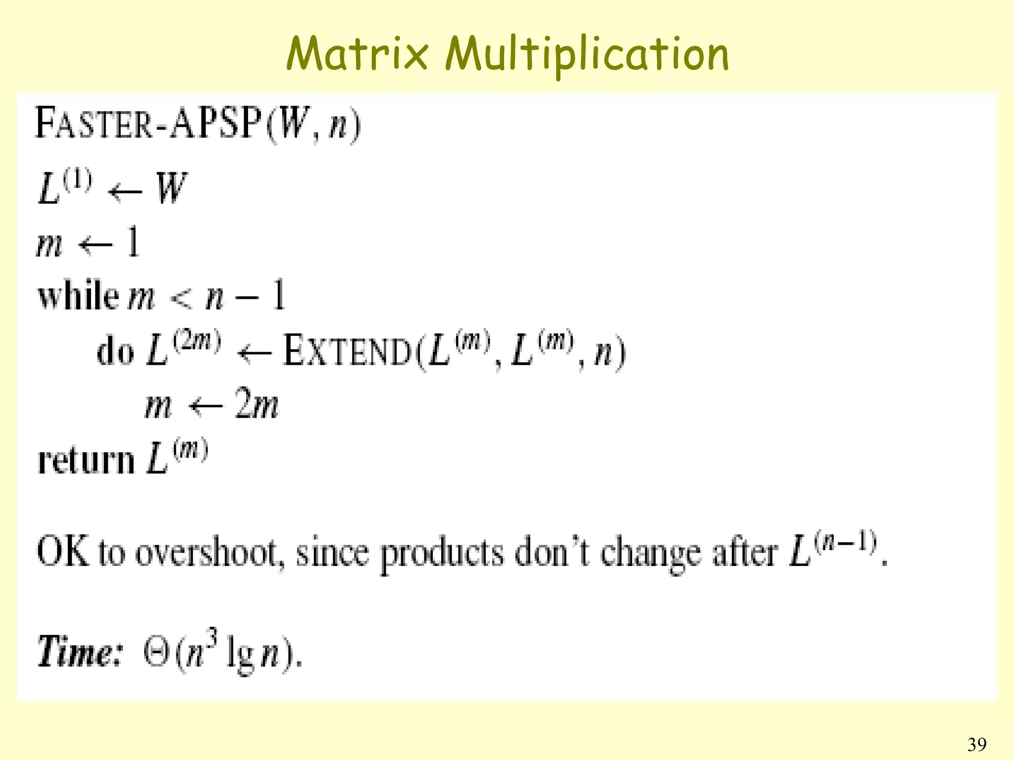
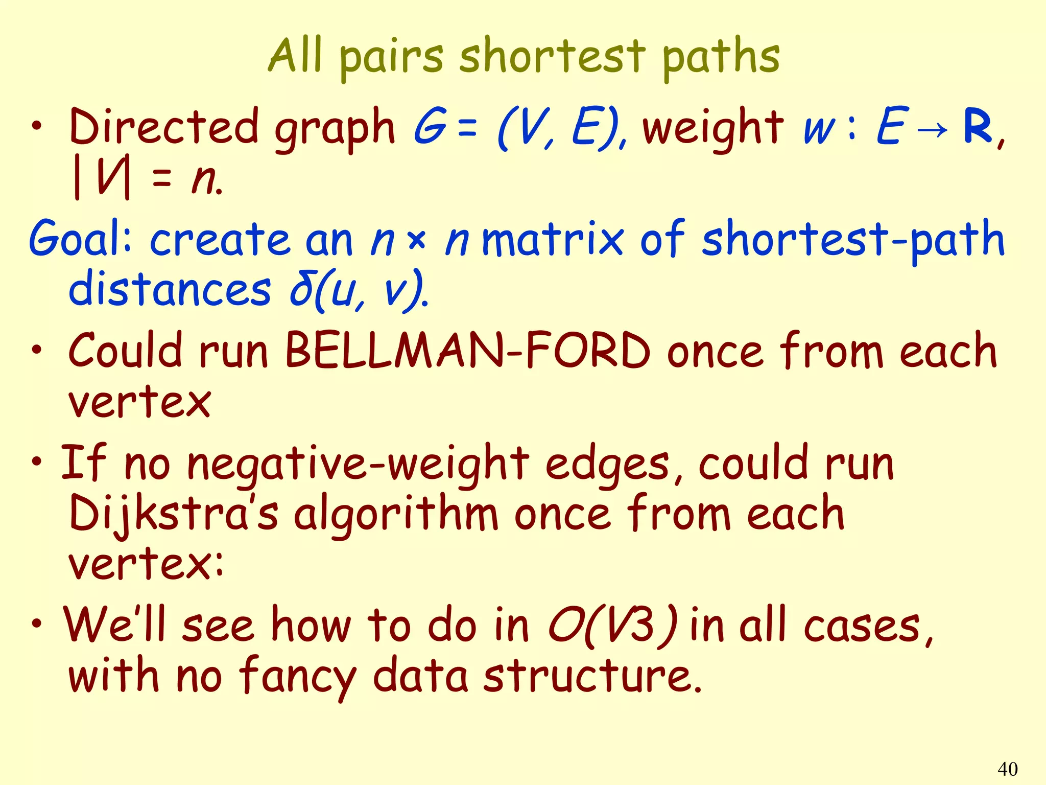
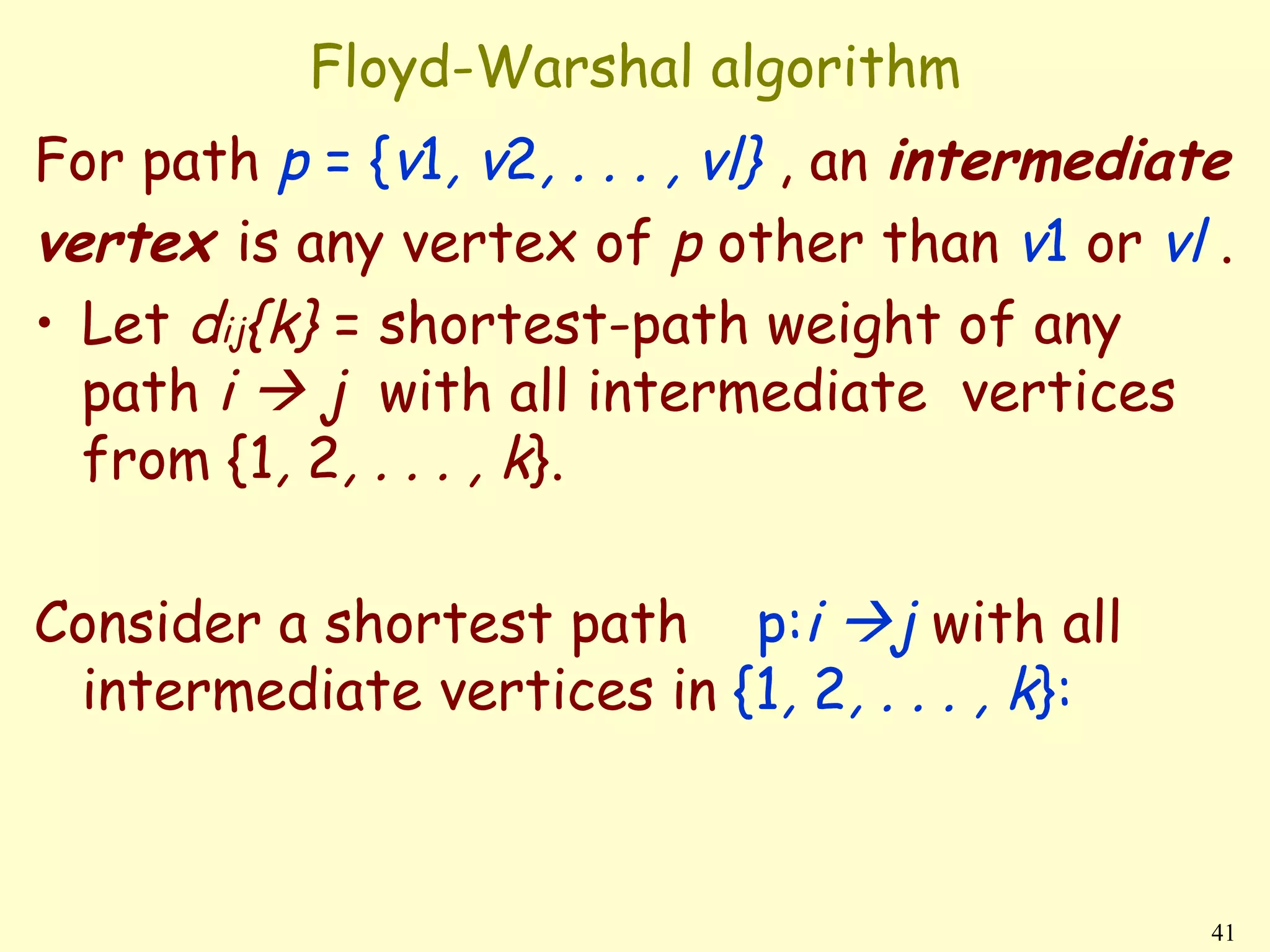
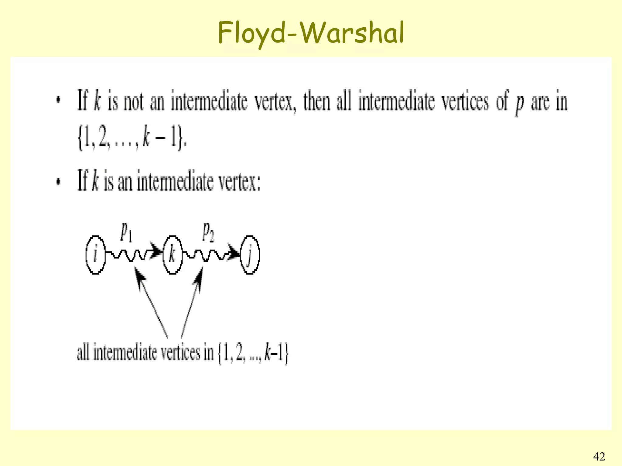
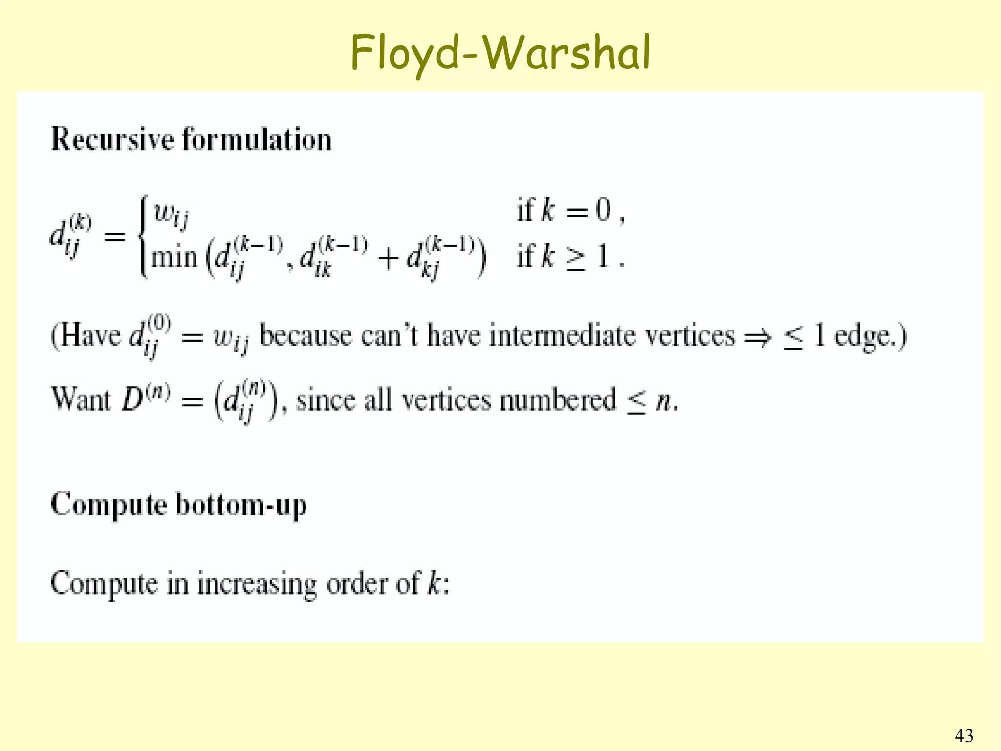
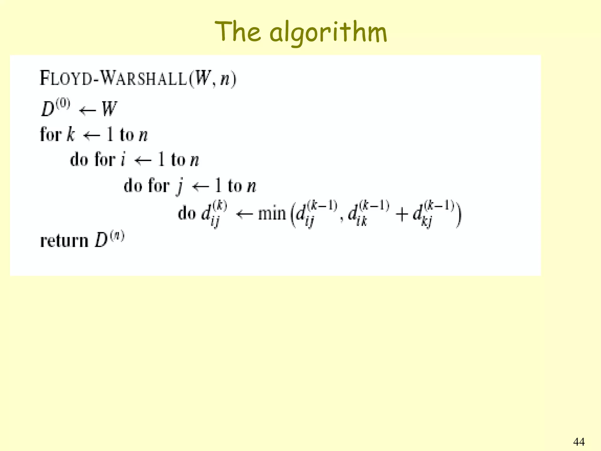
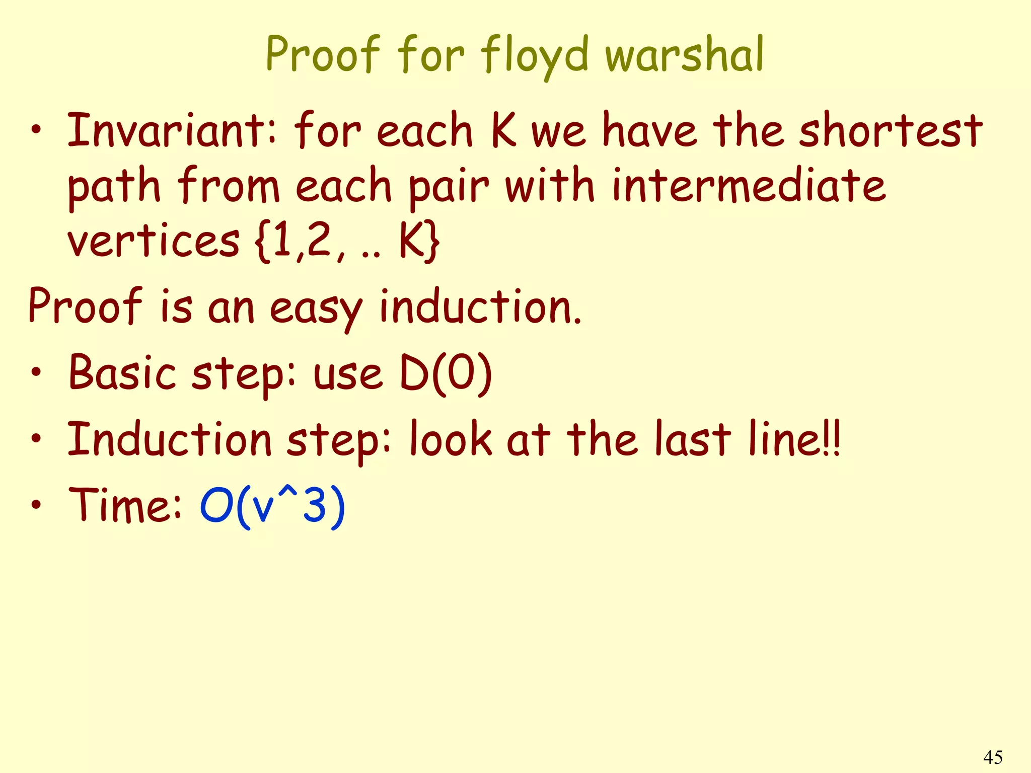
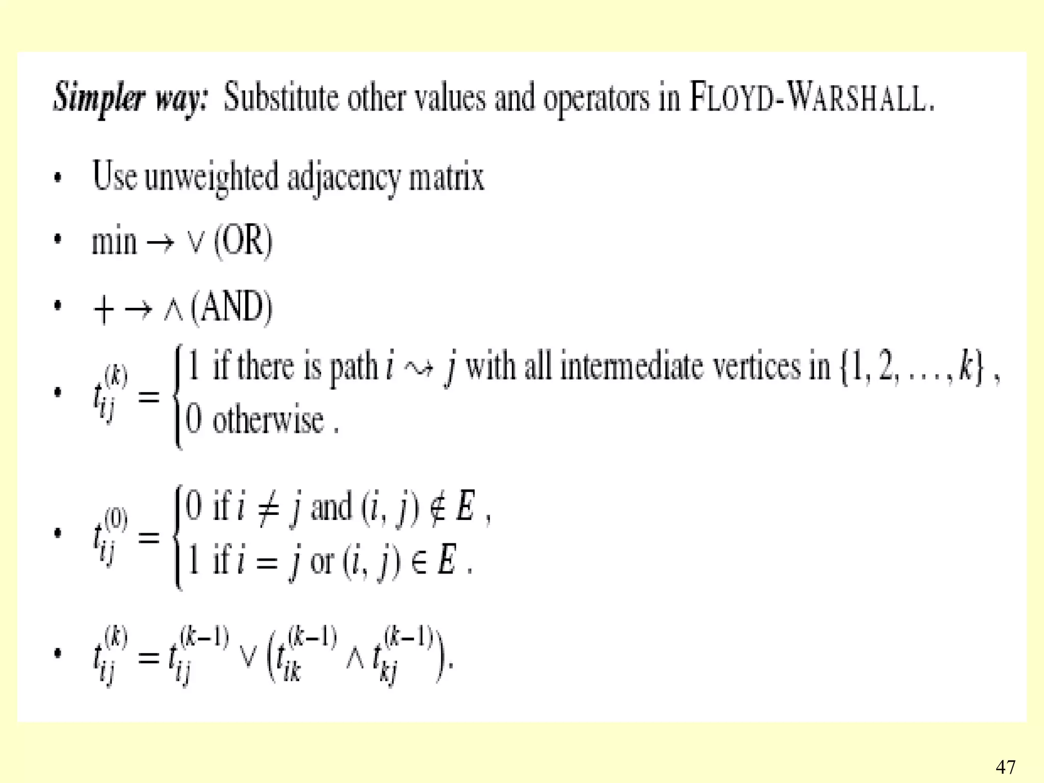
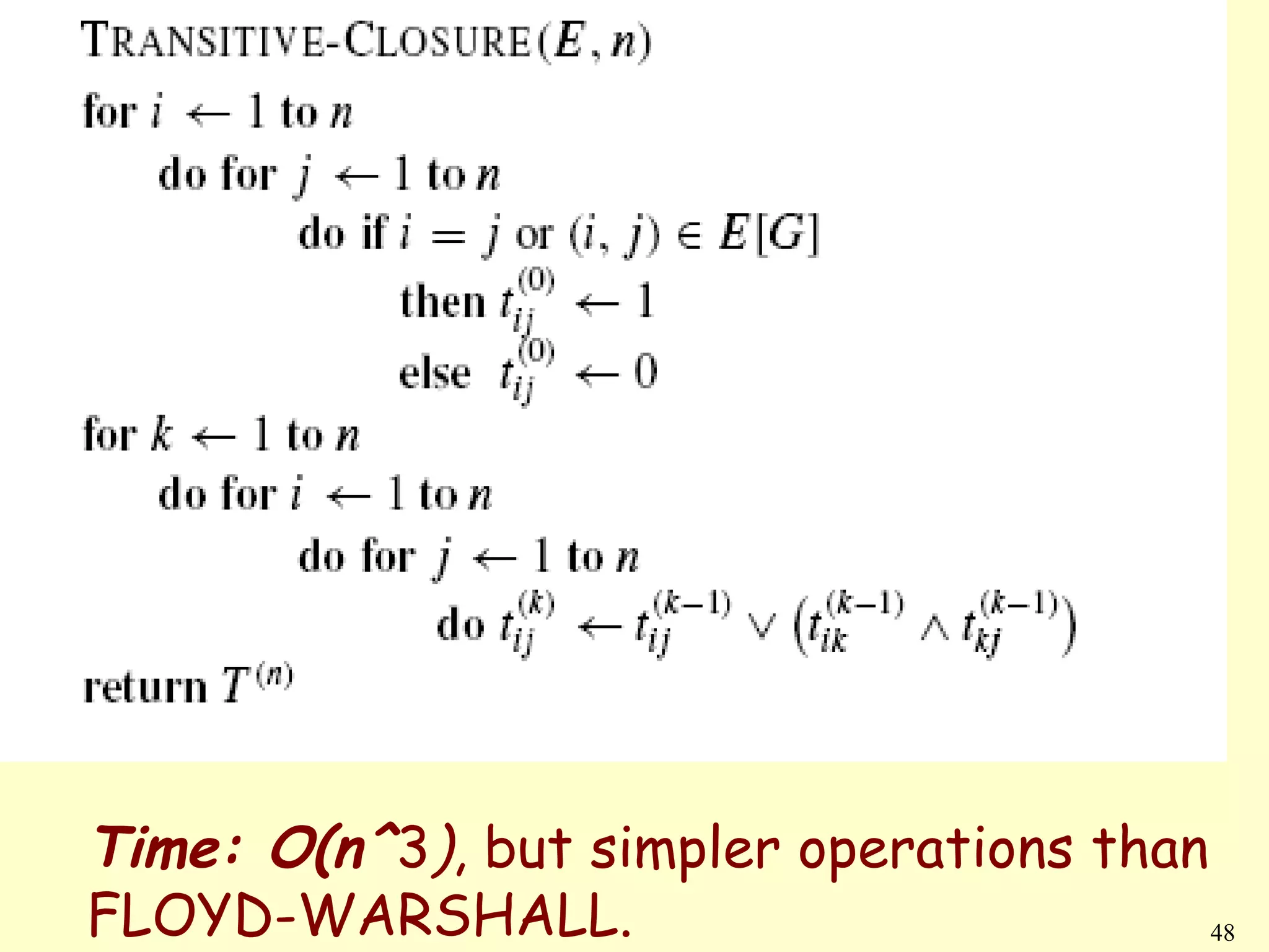
The document discusses shortest path algorithms for graphs. It defines different variants of shortest path problems like single-source, single-destination, and all-pairs shortest paths. It presents algorithms like Bellman-Ford, Dijkstra's algorithm, and Floyd-Warshal algorithm to solve these problems. Bellman-Ford handles negative edge weights but has a higher time complexity of O(V^3) compared to Dijkstra's which only works for positive edges. Floyd-Warshal solves the all-pairs shortest paths problem in O(V^3) time using dynamic programming and matrix multiplication.

1. Shortest paths in graphs
1

2. Shortest path IN directed graph
2

3. Shortest paths
3

4. Variants
• Single-source: Find shortest paths from a
given source vertex s in V to every vertex
v in V.
• Single-destination: Find shortest paths to
a given destination vertex.
• Single-pair: Find shortest path from u to
v. No way known that’s better in worst case
than solving single-source.
• All-pairs: Find shortest path from u to v
for all u, v in V. We’ll see algorithms for all-
pairs in the next chapter.
4

5. Negative-weight edges
• OK, as long as no negative-weight cycles
are reachable from the source.
• •If we have a negative-weight cycle, we can
just keep going around it, and get
• w(s, v) = −∞for all v on the cycle.
• But OK if the negative-weight cycle is not
reachable from the source.
• Some algorithms work only if there are no
negative-weight edges in the graph.
5

6. Lemma 1)
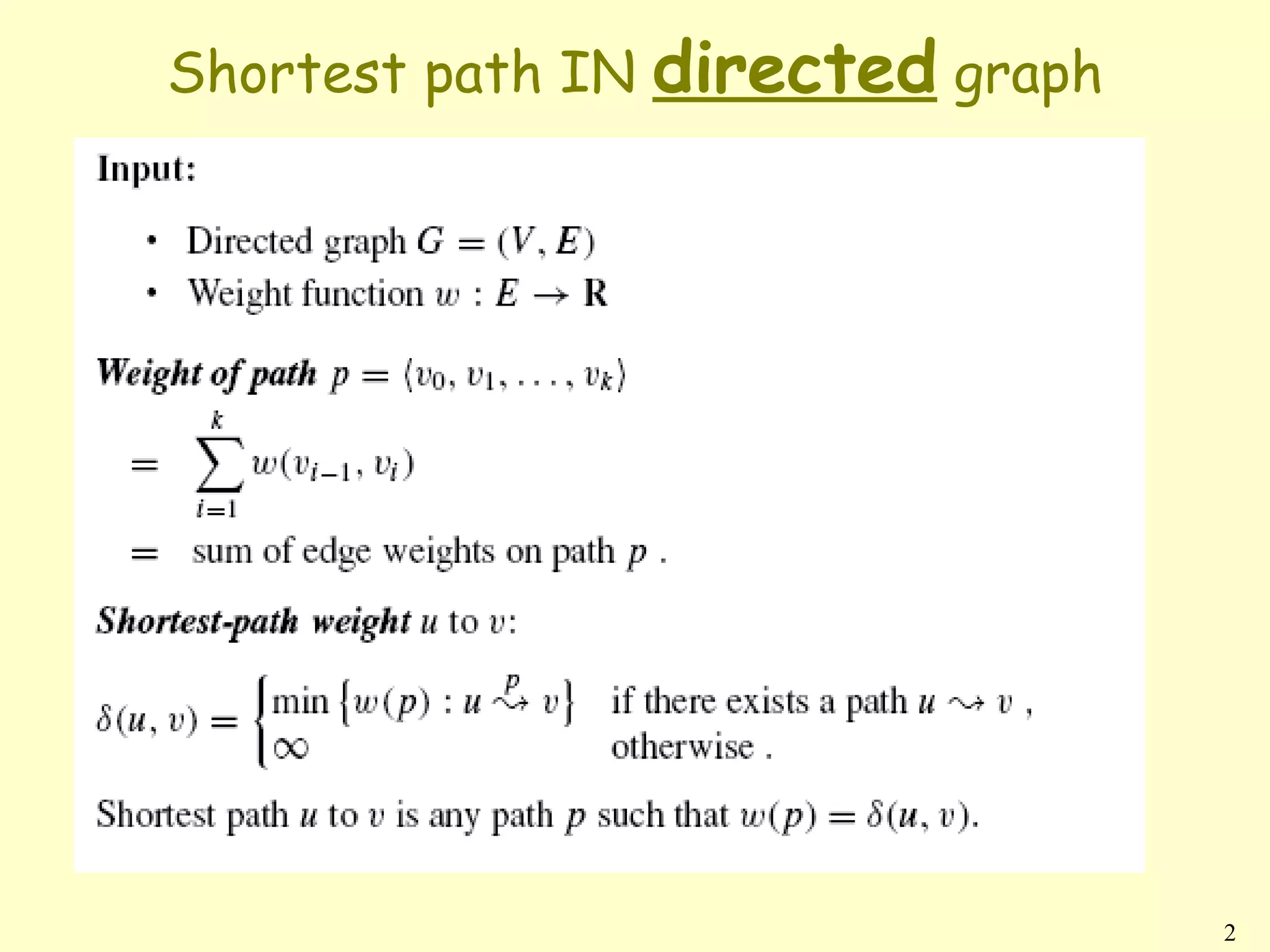
• Optimal substructure lemma: Any sub-path of
a shortest path is a shortest path.
• Shortest paths can’t contain cycles:
proofs: rather trivial.
• We use the d[v] array at all times
INIT-SINGLE-SOURCE(V, s)
{
for each v in V{
d[v]←∞
π[v] ← NIL
}
d[s] ← 0
}
6

7. Relaxing
RELAX(u, v, w){
if d[v] > d[u] + w(u, v) then{
d[v] ← d[u] + w(u, v)
π[v]← u
}
}
For all the single-source shortest-paths
algorithms we’ll do the following:
• start by calling INIT-SINGLE-SOURCE,
• then relax edges.
The algorithms differ in the order and
how many times they relax each edge.
7

8. Lemma 2) Triangle inequality
Claim: For all (u, v) in E, we have
δ(s, v) ≤ δ(s, u) + w(u, v).
Proof: Weight of shortest path s ---> v is
≤ weight of any path s --->v.
Path s ---> u → v is a path s --->v, and if we
use a shortest path s ---> u, its weight is
δ(s, u) + w(u, v).
8

9. Lemma 3) Upper-bound property
1) Always have d[v] ≥ δ(s, v) for all v.
2) Once d[v] = δ(s, v), it never changes.
Proof Initially true.
• Suppose there exists a vertex such that
d[v] < δ(s, v). Without loss of generality, v is first
vertex for which this happens.
• Let u be the vertex that causes d[v] to change.
Then d[v] = d[u] + w(u, v).
So, d[v] < δ(s, v)
≤ δ(s, u) + w(u, v) (triangle inequality)
≤ d[u] + w(u, v) (v is first violation)
 d[v] < d[u] + w(u, v) .
Contradicts d[v] = d[u] + w(u, v).
9

10. Lemma 4: Convergence property
If s ---> u → v is a shortest path and
d[u] = δ(s, u), and we call RELAX(u,v,w), then
d[v] = δ(s, v) afterward.
Proof: After relaxation:
d[v] ≤ d[u] + w(u, v) (RELAX code)
= δ(s, u) + w(u, v) (assumption)
= δ(s, v) (Optimal substructure lemma)
Since d[v] ≥ δ(s, v), must have d[v] = δ(s, v).
10

11. (Lemma 5) Path relaxation property
Let p = v0, v1, . . . , vk be a shortest path from s = v0
to vk .
If we relax, in order, (v0, v1), (v1, v2), . . . , (Vk−1,
Vk), even intermixed with other relaxations,
then d[Vk ] = δ(s, Vk ).
Proof Induction to show that d[vi ] = δ(s, vi ) after
(vi−1, vi ) is relaxed.
Basis: i = 0. Initially, d[v0] = 0 = δ(s, v0) = δ(s, s).
Inductive step: Assume d[vi−1] = δ(s, vi−1). Relax
(vi−1, vi ). By convergence property, d[vi ] = δ(s,
vi ) afterward and d[vi ] never changes.
11

12. The Bellman-Ford algorithm
• Allows negative-weight edges.
• Computes d[v] and π[v] for all v inV.
• Returns TRUE if no negative-weight cycles
reachable from s, FALSE otherwise.
12

13. Bellman-ford
BELLMAN-FORD(V, E, w, s){
INIT-SINGLE-SOURCE(V, s)
for i ← 1 to |V| − 1
for each edge (u, v) in E
RELAX(u, v, w)
for each edge (u, v) in E
if d[v] > d[u] + w(u, v)
return FALSE
return TRUE
}
Time: O(V*E)= O(V^3) in the worst case.
13

14. Correctness of Belman-Ford
Let v be reachable from s, and let p = {v0, v1, . . . , vk}
be a shortest path from s  v,
where v0 = s and vk = v.
• Since p is acyclic, it has ≤ |V| − 1 edges, so k ≤|V|−1.
Each iteration of the for loop relaxes all edges:
• First iteration relaxes (v0, v1).
• Second iteration relaxes (v1, v2).
• kth iteration relaxes (vk−1, vk).
By the path-relaxation property,
d[v] = d[vk ] = δ(s, vk ) = δ(s, v).
14

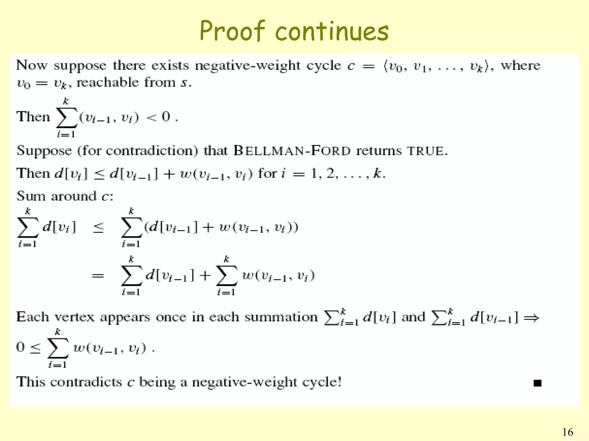
15. How about the TRUE/FALSE return value?
• Suppose there is no negative-weight cycle
reachable from s.
At termination, for all (u, v) in E,
d[v] = δ(s, v)
≤ δ(s, u) + w(u, v) (triangle inequality)
= d[u] + w(u, v) .
So BELLMAN-FORD returns TRUE.
15

16. Proof continues
16

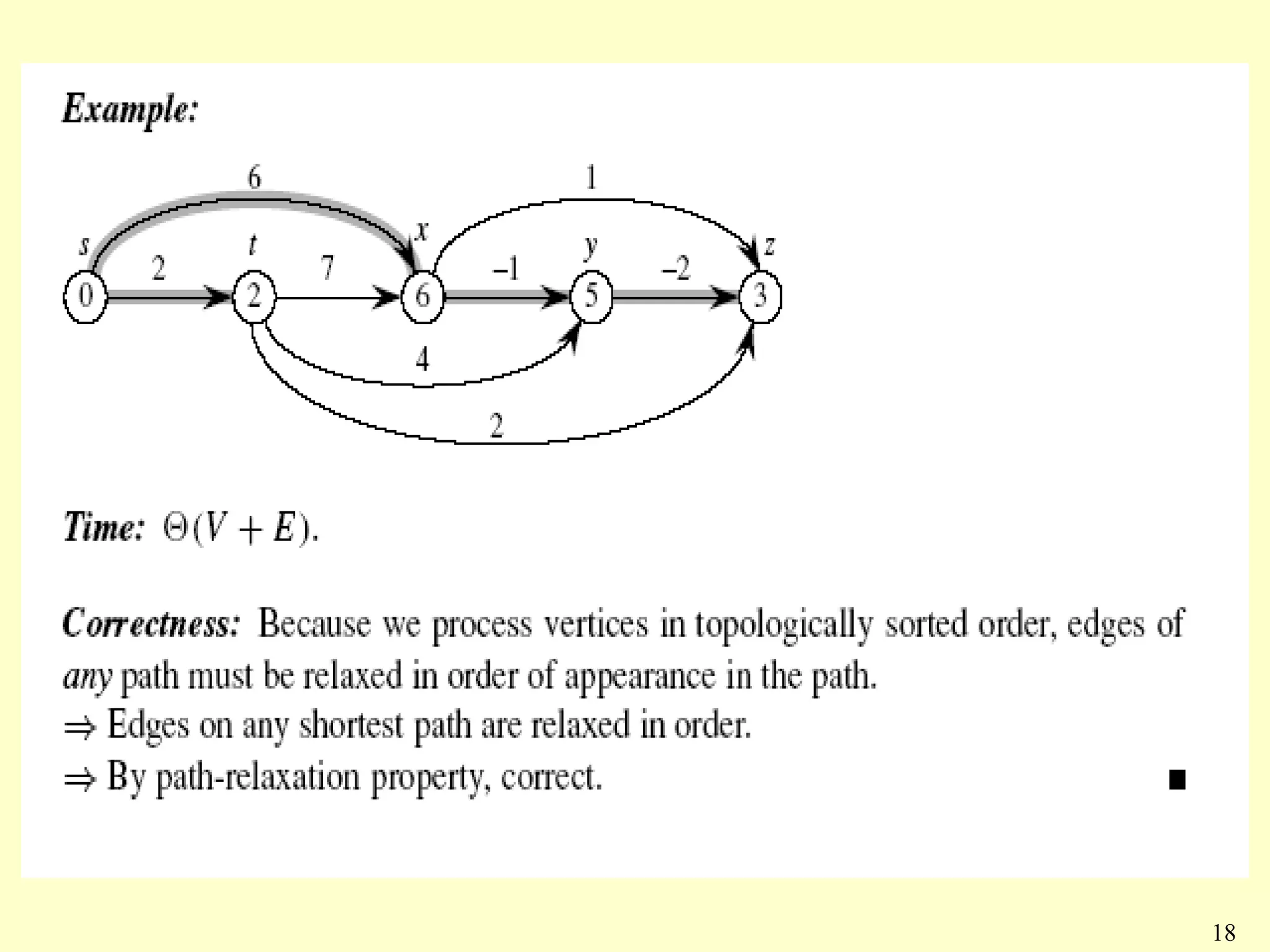
17. Single-source shortest paths in a directed
acyclic graph
DAG-SHORTEST-PATHS(V, E, w, s)
{
topologically sort the vertices
INIT-SINGLE-SOURCE(V, s)
for each vertex u, in topologically order
for each vertex v in Adj[u]
RELAX(u, v, w)
}
17

18. 18

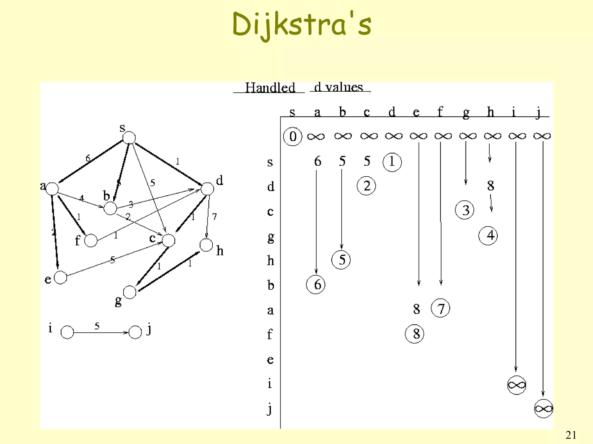
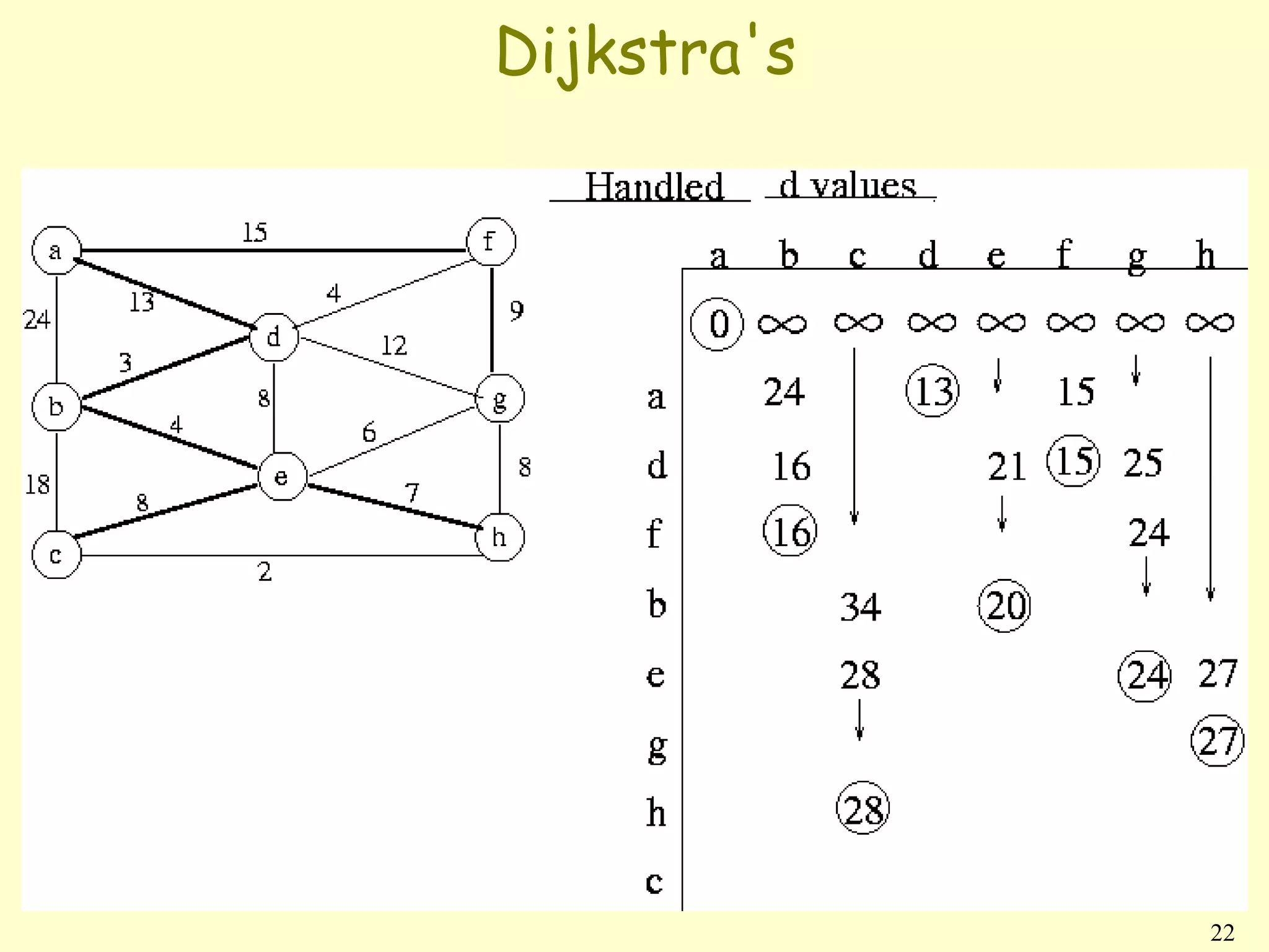
19. Dijkstra’s algorithm
• No negative-weight edges.
• Essentially a weighted version of breadth-
first search.
• Instead of a FIFO queue, uses a priority
queue.
• Keys are shortest-path weights (d[v]).
• Have two sets of vertices:
S = vertices whose final shortest-path
weights are determined,
Q = priority queue = (was V − S. not
anymore)
19

20. Dijkstra algorithm
DIJKSTRA(V, E, w, s){
INIT-SINGLE-SOURCE(V, s)
Q←s
while Q = ∅{
u ← EXTRACT-MIN(Q)
for each vertex v in Adj [u]{
if (d[v] == infinity){
RELAX(u,v,w); (d[v]=d[u]+w[u,v])
enqueue(v,Q)
}
elseif(v inside Q)
RELAX(u,v,w);
change priority(Q,v);
}
} 20

21. Dijkstra's
21

22. Dijkstra's
22

23. Best-first search
• Best first search – an algorithm scheme:
• Have a queue (open-list) of nodes. That is of
generated but no expanded.
• List is sorted according to a cost function.
• Add the start node to the queue
=============================
while queue not empty{ (expansion cycle):
• Remove the best node from the queue
• Goal-test (If goal, stop)
• Add its children to the queue
• Take care of duplicates {relax}
}
23

24. Best-first search
• Best-first search algorithm differ in their
cost function, labeled f(n)
• and maybe some other technical details are
different too.
• There are many implementation variants.
• Breadth-first search: f(n) = number of edges in the tree
• Dijsktra’s algorithm: f(n) = weight of the edges.
• Also called Unifrom cost search (UCS). Should be called
wegihted-breadth-first search (WBRFS).
• A* Algorithm: f(n)=g(n)+h(n). We will study this next year.
• Other special cases too.
24

25. Best-first search
• In general a node n in best-first search is
going through the following three stages:
• Unknown It was not yet generated.
• AKA (free, white, unseen…)
• In queue n was generated and it is in the queue.
• AKA (Opened, generated-not-expanded, touched,
visited, gray, seen-not-handled)
• Expanded (AKA, handled, finished, black,
closed)
25

26. Correctness proof for Dijkstra
• 1) Queue is a perimeter of nodes around s.
• Proof by induction:
• Initially true. S is a perimeter around itself.
• Generalization: A node was removed, but all its negihbours were added.
• Consequence: every path to the goal (including any shortest path)
has a representative node in queue
• 2) The cost of a node in queue can only be increased.
• Proof: Since all edges are non-negative. Cost can only be increased.
• 3) When node is chosen for expansion, its cost is the best in the
queue.
• Consequence: If there is a better path there must be an ancestor
in the q ueue (1) with a better cost (2). This is impossible. (3)
26

27. Correctness proof for Dijkstra
• B will only be expanded if there is no ancestor
of B with small value.
S S
9 8 4
A A 8
3 B 3 B
C C
27

28. Correctness proof for Dijkstra
• What happens if edges are negative?
• Item 2 (lower bound) is no longer true and therefore -
• Costs are not a lower bound and can be later
decreased. Optimality is not guaranteed.
• When node A is selected,
it does not have the C
shortest path to it. 2
• Why? Because via B we A -4 B
have a shorter path
5 8
• Could be corrected if we
re-insert nodes into the S
queue
28

29. Proof according to book:
very hard and not necessary (Do not learn)
29

30. 30

31. Proof
31

32. All pairs Shortest paths
32

33. 33

34. 34

35. 35

36. APSP
36

37. Matrixes
Observation: EXTEND is like matrix
multiplication:
L→A
W→B
L’ → C
min → +
+→·
∞→0
37

38. C=BxA  L’=LxW
38

39. Matrix Multiplication
39

40. All pairs shortest paths
• Directed graph G = (V, E), weight w : E → R,
|V | = n .
Goal: create an n × n matrix of shortest-path
distances δ(u, v).
• Could run BELLMAN-FORD once from each
vertex
• If no negative-weight edges, could run
Dijkstra’s algorithm once from each
vertex:
• We’ll see how to do in O(V3) in all cases,
with no fancy data structure.
40

41. Floyd-Warshal algorithm
For path p = {v1, v2, . . . , vl} , an intermediate
vertex is any vertex of p other than v1 or vl .
• Let dij{k} = shortest-path weight of any
path i  j with all intermediate vertices
from {1, 2, . . . , k}.
Consider a shortest path p:i j with all
intermediate vertices in {1, 2, . . . , k}:
41

42. Floyd-Warshal
42

43. Floyd-Warshal
43

44. The algorithm
44

45. Proof for floyd warshal
• Invariant: for each K we have the shortest
path from each pair with intermediate
vertices {1,2, .. K}
Proof is an easy induction.
• Basic step: use D(0)
• Induction step: look at the last line!!
• Time: O(v^3)
45

46. Transitive closure
Given G = (V, E), directed.
Compute G∗ = (V, E∗).
• E∗ = {(i, j ) : there is a path i  j in G}.
Could assign weight of 1 to each edge, then
run FLOYD-WARSHALL.
• If di j < n, then there is a path i  j .
• Otherwise, di j =∞ and there is no path.
46

47. 47

48. Time: O(n^3), but simpler operations than
FLOYD-WARSHALL. 48