Bellman ford algorithm

1
SINGLE-SOURCE SHORTEST PATHS

2
Introduction
Generalization of BFS to handle weighted graphs
• Direct Graph G = ( V, E ), edge weight fn ; w : E → R
• In BFS w(e)=1 for all e  E
Weight of path p = v1  v2  …  vk is
1
1
1
( ) ( , )
k
i i
i
w p w v v



 

3
Shortest Path
Shortest Path = Path of minimum weight
δ(u,v)= min{ω(p) : u v}; if there is a path from u to v,
 otherwise.
p

4
Shortest-Path Variants
• Shortest-Path problems
– Single-source shortest-paths problem: Find the shortest path from s
to each vertex v. (e.g. BFS)
– Single-destination shortest-paths problem: Find a shortest path to a
given destination vertex t from each vertex v.
– Single-pair shortest-path problem: Find a shortest path from u to v
for given vertices u and v.
– All-pairs shortest-paths problem: Find a shortest path from u to v
for every pair of vertices u and v.

5
Optimal Substructure Property
Theorem: Subpaths of shortest paths are also shortest paths
• Let P1k = <v1, ... ,vk > be a shortest path from v1 to vk
• Let Pij = <vi, ... ,vj > be subpath of P1k from vi to vj
for any i, j
• Then Pij is a shortest path from vi to vj

6
Proof: By cut and paste
• If some subpath were not a shortest path
• We could substitute a shorter subpath to create a shorter
total path
• Hence, the original path would not be shortest path
v2
v3 v4
v5 v6 v7
v1
v0

7
Definition:
• δ(u,v) = weight of the shortest path(s) from u to v
Well Definedness:
• negative-weight cycle in graph: Some shortest paths may not
be defined
• argument:can always get a shorter path by going around the
cycle again
s v
cycle
< 0

8
Negative-weight edges
• No problem, as long as no negative-weight cycles are
reachable from the source
• Otherwise, we can just keep going around it, and
get w(s, v) = −∞ for all v on the cycle.

9
Triangle Inequality
Lemma 1: for a given vertex s  V and for every edge (u,v)  E,
• δ(s,v) ≤ δ(s,u) + w(u,v)
Proof: shortest path s v is no longer than any other path.
• in particular the path that takes the shortest path s v and
then takes cycle (u,v)
s
u v

10
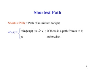
Relaxation
• Maintain d[v] for each v  V
• d[v] is called shortest-path weight estimate
and it is upper bound on δ(s,v)
INIT(G, s)
for each v  V do
d[v] ← ∞
π[v] ← NIL
d[s] ← 0

11
Relaxation
RELAX(u, v)
if d[v] > d[u]+w(u,v) then
d[v] ← d[u]+w(u,v)
π[v] ← u
5
u v
v
u
2
2
9
5 7
Relax(u,v)
5
u v
v
u
2
2
6
5 6

12
Properties of Relaxation
Algorithms differ in
 how many times they relax each edge, and
 the order in which they relax edges
Question: How many times each edge is relaxed in BFS?
Answer: Only once!

13
Given:
• An edge weighted directed graph G = ( V, E ) with edge
weight function (w:E → R) and a source vertex s  V
• G is initialized by INIT( G , s )
Lemma 2: Immediately after relaxing edge (u,v),
d[v] ≤ d[u] +w(u,v)
Lemma 3: For any sequence of relaxation steps over E,
(a) the invariant d[v] ≥ δ(s,v) is maintained
(b) once d[v] achieves its lower bound, it never changes.

14
Proof of (a): certainly true after
INIT(G,s) : d[s] = 0 = δ(s,s):d[v] = ∞ ≥ δ(s,v)  v V-{s}
• Proof by contradiction:Let v be the first vertex for which
RELAX(u, v) causes d[v] < δ(s, v)
• After RELAX(u , v) we have
• d[u] + w(u,v) = d[v] < δ(s, v)
≤ δ(s, u) + w(u,v) by L1
• d[u]+w(u,v) < δ(s, u) + w(u, v) => d[u] < δ(s, u)
contradicting the assumption

15
Proof of (b):
• d[v] cannot decrease after achieving its lower bound;
because d[v] ≥ δ(s,v)
• d[v] cannot increase since relaxations don’t increase d
values.

16
C1 : For any vertex v which is not reachable from s, we have
invariant d[v] = δ(s,v) that is maintained over any sequence of
relaxations
Proof: By L3(b), we always have ∞ = δ(s,v) ≤ d[v]
=> d[v] = ∞ = δ(s,v)

17
Lemma 4: Let s u →v be a shortest path from s to v for
some u,v  V
• Suppose that a sequence of relaxations including
RELAX(u,v) were performed on E
• If d[u] = δ(s, u) at any time prior to RELAX(u, v)
• then d[v] = δ(s, v) at all times after RELAX(u, v)

18
Proof: If d[u] = δ(s, v) prior to RELAX(u, v)
d[u] = δ(s, v) hold thereafter by L3(b)
• After RELAX(u,v), we have d[v] ≤ d[u] + w(u, v) by L2
= δ(s, u) + w(u, v) hypothesis
= δ(s, u) by optimal subst.property
• Thus d[v] ≤ δ(s, v)
• But d[v] ≥ δ(s, v) by L3(a) => d[v] = δ(s, v)
Q.E.D.

19
Single-Source Shortest Paths in DAGs
• Shortest paths are always well-defined in dags
 no cycles => no negative-weight cycles even if
there are negative-weight edges
• Idea: If we were lucky
 To process vertices on each shortest path from left
to right, we would be done in 1 pass due to L4

20
In a dag:
• Every path is a subsequence of the topologically sorted
vertex order
• If we do topological sort and process vertices in that order
• We will process each path in forward order
 Never relax edges out of a vertex until have processed
all edges into the vertex
• Thus, just 1 pass is sufficient

21
DAG-SHORTEST PATHS(G, s)
TOPOLOGICALLY-SORT the vertices of G
INIT(G, s)
for each vertex u taken in topologically sorted order do
for each v  Adj[u] do
RELAX(u, v)

Runs in linear time: Θ(V+E)
 topological sort: Θ(V+E)
 initialization: Θ(V+E)
 for-loop: Θ(V+E)
each vertex processed exactly once
=> each edge processed exactly once: Θ(V+E)

29
Thm: (Correctness of DAG-SHORTEST-PATHS):
At termination of DAG-SHORTEST-PATHS procedure
d[v] = δ(s, v) for all v V

30
Proof: If v  Rs , then d[v] = δ(s, v)
• If v  Rs , so a shortest path
p = <v0=s, v1, v2, …,vk=v>
• Because we process vertices in topologically sorted order
 Edges on p are relaxed in the order
(u0, u1),(u1, u2),...,(uk-1, uk)
• A simple induction on k using L4 shows that
 d[vi] = δ(s, v) at termination for i = 0,1,2,...,k
v  V

31
• Non-negative edge weight
• Like BFS: If all edge weights are equal, then use BFS,
otherwise use this algorithm
• Use Q = priority queue keyed on d[v] values
(note: BFS uses FIFO)
Dijkstra’s Algorithm For Shortest Paths

32
DIJKSTRA(G, s)
INIT(G, s)
S←Ø > set of discovered nodes
Q←V[G]
while Q ≠Ø do
u←EXTRACT-MIN(Q)
S←S U {u}
for each v  Adj[u] do
RELAX(u, v) > May cause
> DECREASE-KEY(Q, v, d[v])

33
Example
3
 
 
0
s
u v
y
x
10
5
1
2 9
4 6
7
2

34
Example
2
10 
5 
0
s
u v
y
x
10
5
1
3
9
4 6
7
2

35
Example
2
8 14
5 7
0
s
y
x
10
5
1
3 9
4 6
7
2
u v

36
Example
10
8 13
5 7
0
s
u v
y
x
5
1
2 3 9
4 6
7
2

37
Example
8
u v
9
5 7
0
y
x
10
5
1
2 3 9
4 6
7
2
s

38
Example
u
5
8 9
5 7
0
v
y
x
10
1
2 3 9
4 6
7
2
s

39
Observe :
• Each vertex is extracted from Q and inserted into S
exactly once
• Each edge is relaxed exactly once
• S = set of vertices whose final shortest paths have already
been determined
 i.e. , S = {v  V: d[v] = δ(s, v) ≠ ∞ }

40
• Similar to BFS algorithm: S corresponds to the set of
black vertices in BFS which have their correct breadth-
first distances already computed
• Greedy strategy: Always chooses the closest(lightest)
vertex in Q = V-S to insert into S
• Relaxation may reset d[v] values thus updating
Q = DECREASE-KEY operation.

41
• Similar to Prim’s MST algorithm: Both algorithms
use a priority queue to find the lightest vertex outside a
given set S
• Insert this vertex into the set
• Adjust weights of remaining adjacent vertices outside the
set accordingly

42
Example: Run algorithm on a sample graph
4
3
2
10
5 1
s
0
∞ 5
∞ 10 9 8
∞ 6

43
Thm: At termination of Dijkstra’s algorithm
d[u] = δ(s, u)  u  V
Proof: Trivial for u  Rs since d[u] = ∞ = δ(s, u)
Proof: By contradiction for u  Rs
• Let u be the first vertex for which d[u] ≠ δ(s, u) when it is
inserted to S
• d[u] > δ(s, u) since d[v] ≥ δ(s, v)  v  V by L3(a)
• Consider an actual shortest path p from s  S to
u  Q = V-S
Correctness of Dijkstra’s Algorithm

44
• Let y be first vertex along p such that y  V-S
• Let x  V be y’s predecessor along p
• Thus p can be decomposed as s x→y u
Claim: d[y] = δ(s, y) when u was selected from Q for
insertion into S
• Observe that x  S by assumption on y
• d[x] = δ(s, x) by assumption on u being first
vertex in S for which d[u] ≠ δ(s, u)
p1 p2

45
• x  S => x is already processed => edge (x, y) is already
relaxed => d[y] = δ(s, y) by L4 & optimal subst. property
s
x y
u
P2
P1

46
• d[u] > δ(s, u)
= δ(s, y) + w(p2) by optimal substructure Thm
= d[y] + w(p2) by the above claim
≥ d[y] due to non-negative edge-weight assumption
• d[u] > d[y] => algorithm would have chosen y to
process next, not u.Contradiction
s
x y
u
P2
P1

47
Figure about the proof:
s
x y
u
P2
P1
S
 vertices x&y are distinct, but may have s=x and/or y=u
 path P2 may or may not reenter set S

48
• Look at different Q implementation, as did for Prim’s
algorithm
• Initialization (INIT) : Θ(V) time
• While-loop:
• EXTRACT-MIN executed |V| times
• DECREASE-KEY executed |E| times
• Time T = |V| x TE-MIN +|E| x TD-KEY
Running Time Analysis of
Dijkstra’s Algorithm

49
Look at different Q implementation, as did for Prim’s
algorithm
Q TE-MIN TD-KEY TOTAL
• Linear
Unsorted O(V) O(1) O(V²+E)
Array:
• Binary Heap: O(lgV) O(logV) O(VlgV+ElgV) = O(ElgV)
• Fibonacci heap: O(lgV) O(1) O(VlgV+E)
(Amortized) (Amortized) (Worst Case)

50
Q = unsorted-linear array:
• Scan the whole array for EXTRACT-MIN
• Joint index for DECREASE-KEY
Q = Fibonacci heap: note advantage of amortized analysis
• Can use amortized Fibonacci heap bounds per operation
in the analysis as if they were worst-case bound
• Still get (real) worst-case bounds on aggregate running
time

51
Bellman-Ford Algorithm for Single
Source Shortest Paths
• More general than Dijkstra’s algorithm:
 Edge-weights can be negative
• Detects the existence of negative-weight cycle(s)
reachable from s.

52
BELMAN-FORD( G, s )
INIT( G, s )
for i ←1 to |V|-1 do
for each edge (u, v)  E do
RELAX( u, v )
for each edge ( u, v )  E do
if d[v] > d[u]+w(u,v) then
return FALSE > neg-weight cycle
return TRUE

53
Observe:
• First nested for-loop performs |V|-1 relaxation passes;
relax every edge at each pass
• Last for-loop checks the existence of a negative-weight
cycle reachable from s

54
• Running time = O(VxE)
Constants are good; it’s simple, short code(very
practical)
• Example: Run algorithm on a sample graph with
no negative weight cycles.

55
Bellman-Ford Algorithm
Example
5
 
 
0
s
z
y
6
7
8
-3
7
2
9
-2
x
t
-4

56
Example
6 
7 
0
s
z
y
6
7
8
-3
7
2
9
-2
x
t
-4
5

57
Example
6 4
7 2
0
s
z
y
6
7
8
-3
7
2
9
-2
x
t
-4
5

58
Example
2 4
7 2
0
s
z
y
6
7
8
-3
7
2
9
-2
x
t
-4
5

59
Example
2 4
7 2
0
s
z
y
6
7
8
-3
7
2
9
-2
x
t
-4
5

60
• Converges in just 2 relaxation passes
• Values you get on each pass & how early converges
depend on edge process order
• d value of a vertex may be updated more than once in a
pass

61
Correctness of Bellman-Ford Algorithm
L5: Assume that G contains no negative-weight cycles
reachable from s
• Thm, at termination of BELLMAN-FORD, we have
d[v] = δ(s, v)  v Rs
• Proof: Let v  Rs , consider a shortest path
p = <v0=s,v1,v2,...,vk=v> from s to v

62
• No neg-weight cycle => path p is simple => k ≤|V|-1
o i.e., longest simple path has |V|-1 edge
prove by induction that for i = 0,1,...,k
o we have d[v1] = δ(s,vi) after i-th pass and this
equality maintained thereafter
basis: d[v0=s] = 0 = δ(s, s) after INIT( G, s ) and doesn’t
change by L3(b)
hypothesis: assume that d[vi-1] = δ(s,vi-1) after the (i-1)th
pass

63
• Edge (vi-1, vi) is relaxed in the ith pass
o so by L4 , d[vi] = δ(s,vi) after i-th pass, and doesn’t
change thereafter
Thm:Bellman-Ford algorithm
(a) returns TRUE together with correct d values, if G
contains no neg-weight cycle  Rs
(b) returns FALSE, otherwise

64
Proof of (a):
• if v  Rs , then L5 proves this claim
• if v  Rs , the claim follows from L1
• Now, prove the claim that BELLMAN-FORD returns
TRUE

65
• At termination, we have for all edges (u, v)  E
d[v] = δ(s,v)
≤ δ(s, u) + w(u, v) by triangle inequality
= d[u] + w(u,v) by first claim proven
• d[v] ≤ d[u] +w(u, v) => none of the if tests in the 2nd for
loop passes therefore, it returns TRUE.

66
k
i = 1
k
i = 1
k
i = 1
k
i = 1

67
But, each vertex in c appears exactly once in both
Σ d[vi] & Σ d[vi-1]
• Therefore, Σ d[vi] = Σ d[vi-1]
• Moreover, d[vi] is finite  vi  C , since c  Rs
• Thus, 0 ≤ Σ w(vi-1, vi)
0 ≤ Σ w(vi-1, vi) = w(c), contradicting w(c) < 0
Q.E.D.
k
i = 1
k
i = 1
k
i = 1
k
i = 1
k
i = 1
k
i = 1

68
LINEAR PROGRAMMING(LP)
• given: an mxn constraint matrix A & an mx1 bound vector b
& an nx1 cost vector c
• problem : find an n-vector x that maximizes cTx subject
•
A ≤ maximizing
A x b C
x n
T
m
n
n
Linear Programming and
m
n

69
• Linear feasibility:
• satisfy m linear constraints : Σ aij ≤ bi
for i = 1,2,...,m
• Linear optimization:
• maximize the linear cost(objective) function: Σ ljxj
• General algorithms:
• simplex: practical, but worst-case is exponential
• ellipsoid: theoretical, polynomial time
• Karmarkar: polynomial time, practical
n
i = 1
n
i = 1

70
Linear Feasibility Problem
• special case of LP
• no optimization criteria
• find x  R such that Ax ≤ b
Systems of Difference Constraints
• special case of linear feasibility problem
• each row of A contains exactly one 1 and one –1, and the
rest 0
• thus, constraints have the form xj-xi ≤ bk ,
1 ≤ i, j ≤ n & 1 ≤ k ≤ m
n

71
x1
x2
x3
x4
≤
0
-1
1
5
4
-1
-3
-3
x1-x2 ≤ 0 = b1
x1-x5 ≤ -1 = b2
x2-x5 ≤ 1 = b3
x3-x1 ≤ 5 = b4
x4-x1 ≤ 4 = b5
x4-x3 ≤ -1 = b6
x5-x3 ≤ -3 = b7
x5-x4 ≤ -3 = b8
x5
example:
1 -1 0 0 0
1 0 0 0 -1
0 1 0 0 -1
-1 0 1 0 0
-1 0 0 1 0
0 0 -1 1 0
0 0 -1 0 1
0 0 0 -1 1
1 2 3 4 5
1
2
3
4
5
6
7
8

72
• Two solutions : x = ( -5, -3, 0,-1, -4 ) & x = < 0, 2, 5, 4, 1 >
note : x = x*+5
• L1: let x = ( x1, x2, ... , xn ) be a solution to a system Ax ≤ b
of difference constraints
=> x+d = (x1+d, x2+d, ..., xn+d) is also a solution for any
constant d
1 2 3 4 5 1 2 3 4 5

73
• proof: for each xi&xj: (xj+d)-(xi+d) = xj-xi
• application: job(task scheduling)
• given: n tasks t1,t2,...,tn
• problem: determine starting time xi for job ti
for i = 1,2,...,n
• constraints:
o xi ≥ xj +dj = duration of tj, i.e., do job ti after
finishing tj
o xi ≤ xj+gij;gj = max permissible time gap between
starting jobs
Q.E.D.

74
• graph theoritical representation of difference constraints
• a system Ax ≤ b of difference constraints with an mxn
constraint matrix A
=> incidence matrix of an edge-weighted directed graph
with n vertices and m edges
• one vertex per variable: V = {v1,v2,...,vn} such that
Vi ↔ Xi for i = 1,2,...,n

75
• one edge per constraint:
k-th constraint xj-xi ≤ bk
• xj-xi ≤ bk edge lij incident to vj(+1)
from vi(-1)
• more than one constraint on xj-xi for a single i,j pair
o :can avoid multiple edges by removing
weaker constraints
vi vj
vi vj

76
• constraint graph for the sample system of difference
constraints
v5
v4 v3
v2
b3 = 1
5 = b4
-3 = b7
4 = b5
b6 = -1
b7 = -3
v1
• constraint graph for the sample system of difference
constraints
1 -1 0 0 0
1 0 0 0 -1
0 1 0 0 -1
-1 0 1 0 0
-1 0 0 1 0
0 0 -1 1 0
0 0 -1 0 1
0 0 0 -1 1
1 2 3 4 5
1
2
3
4
5
6
7
8
0
-1
1
5
4
-1
-3
-3
b

77
• adding vertex s to enable Bellman-Ford algorithm solve the
feasibility problem.
δ(s,vi)
x = (-5, -3, 0, -1, -4)
feasible soln.
1 2 3 4 5
vi
0
0
-1
-3
0
-1 0
-3
s
v5
v1
v2
v3
5
-3
4
-1
1
0
-4
-5
0
0

78
Difference Constraints and
• Thm: let G = (V,E) be the constraint graph of the system
Ax ≤ b of difference constraints.
(a) if G has a neg-wgt cycle then Ax ≤ b has no feasible soln
(b) if G has no neg-wgt cycle then Ax ≤ b has a feasible
solution
• proof(a): let neg-wgt cycle be c = <v1,v2,...,vk=vl>
cycle c contains the following k constraints (inequalities)

79
• x2-x1 ≤ w12
x3-x2 ≤ w23
.
.
.
xk-1-xk-2 ≤ wk-2, k-1
+ xk = x1-xk-1 ≤ wk-1, 1
x1 – x1 ≤ w(i) < 0 => x1-x1 < 0 => no solution

80
• Consider any feasible soln. x for Ax ≤ b
o x must satisfy each of these k inequalities
o x must also satisfy the inequality that results when we
sum them together

81
• proof(b): add vertex s  V with 0-weight edge to each vertex
vi  V
• i.e., G0 = (V0, E0) V0 = V U {S} &
E0 = E U {(s, vi): }&  v V w(s,vi) = 0
• no neg-wgt cycle introduced , because no path to
vertex s
• use Bellman-Ford to find shortest-path weights from
common source s to every Vi V

82
• Claim : X = (xi) with xi = δ(s,vi) is a feasible soln. to Ax ≤ b
o consider kth constraint xj-xi ≤ bk => (vi, vj)  E
with wij = bk
triangle ineaquality: δ(s,vi) ≤ δ(s,vi)+wij
xj ≤ xi + bk
xj - xi ≤ bk
s
vi vj

83
• δ(s,vj) ≤ δ(s,vi) + bk => δ(s,vj) - δ(s,vi) ≤ bk => xj-xi ≤ bk
• so, Bellman-Ford solves a special case of LP
Bellman-Ford also minimizes Max{xi}-Min{xi}
1 ≤i ≤n 1 ≤i ≤n

Bellman ford algorithm

More Related Content

What's hot

Similar to Bellman ford algorithm

More from Ruchika Sinha

Recently uploaded

Bellman ford algorithm