Downloaded 229 times
![Wavelet Transform for Sparse Representation
[Goupillaud et al., 1984]
In the first, we introduce the wavelet transform (WT) as one of the approaches for
sparse representation. The wavelet transform is given by
W(b, a) =
1
√
a
∞
−∞
f(t)ψ
t − b
a
dt, (1)
where f(t) is a signal, ψ(t) is a wavelet function. There are many kind of wavelets
such as Haar wavelet, Meyer wavelet, Mexican Hat wavelet and Morlet wavelet. In
this research, we use the Complex MORlet wavelet (CMOR) which is given by
ψfb,fc (t) =
1
√
πfb
ei2πfct−(t2
/fb)
. (2)
February 2, 2012 6/26](https://image.slidesharecdn.com/main-120201210932-phpapp02/75/Principal-Component-Analysis-for-Tensor-Analysis-and-EEG-classification-6-2048.jpg)
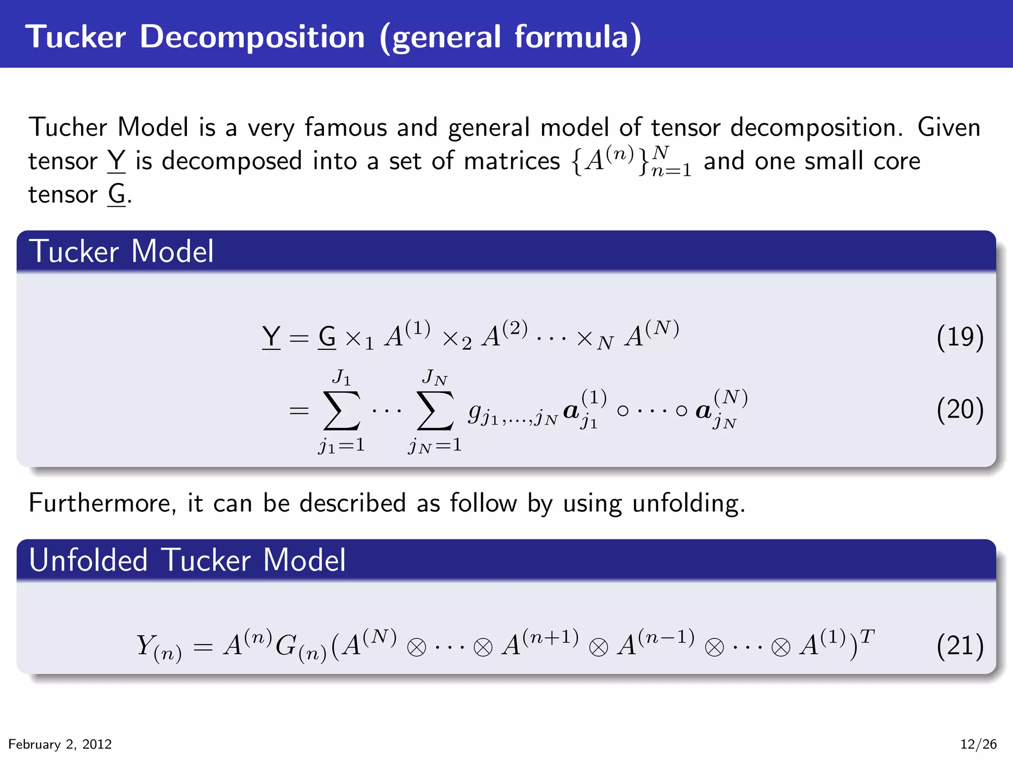
![Kind of Tensor Decomposition [Cichocki et al., 2009]
The degree of freedom of tensor decomposition is very large. So there are many
methods of tensor decomposition. The kind of tensor decomposition is depend on
the constraint. For example, if we constrain the matrices {A(n)
}N
n=1 and the core
tensor G as non-negative matrices and tensor, then this method is the
non-negative tensor factorization (NTF). And if we consider the in-dependency
constraint, then this method is the independent component analysis (ICA). And if
we consider the sparsity constraints, then it is the sparse component analysis
(SCA). And if we consider the orthogonal constraints, then it is the principal
component analysis (PCA).
February 2, 2012 13/26](https://image.slidesharecdn.com/main-120201210932-phpapp02/75/Principal-Component-Analysis-for-Tensor-Analysis-and-EEG-classification-13-2048.jpg)
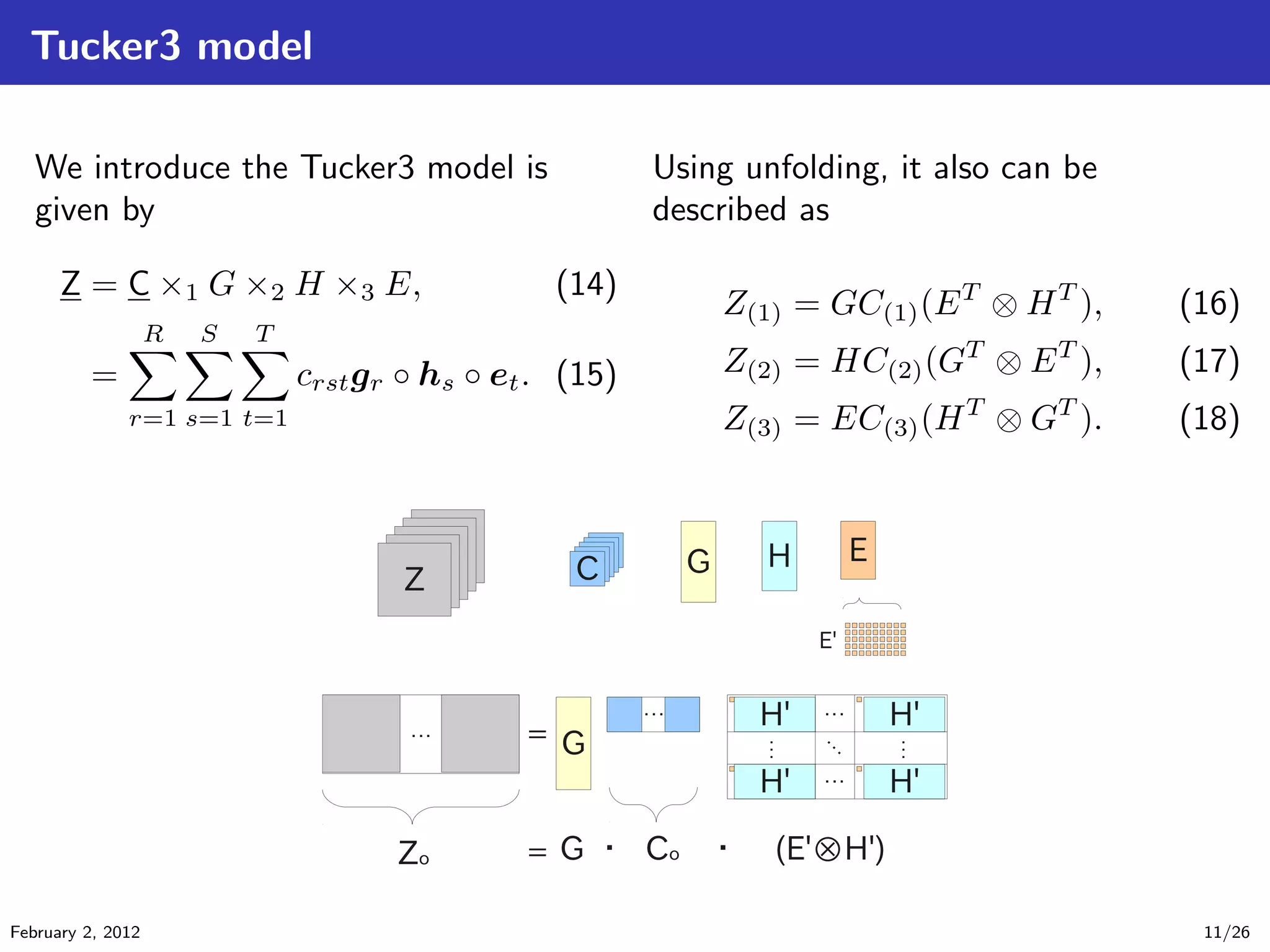
![Principal Component Analysis
[Kroonenberg and de Leeuw, 1980] [Henrion, 1994]
Principal Component Analysis (PCA) is very typical method for signal analysis. In
this slide, we explain PCA in case of 3d-tensor decomposition. The tensor
decomposition model is given by
Z = C ×1 G ×2 H ×3 E. (22)
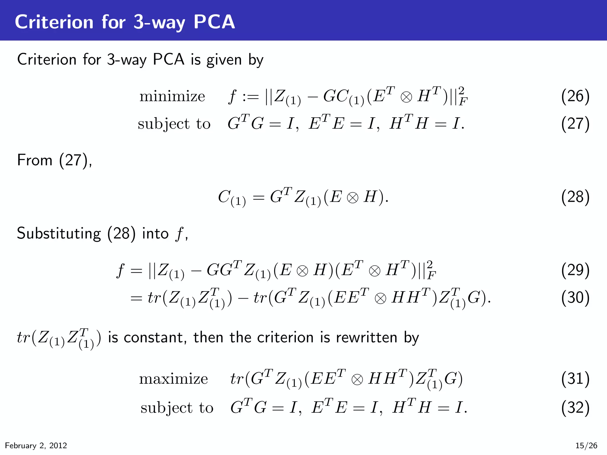
And the criterion of PCA is given by
.
Criterion for PCA
..
.
. ..
.
.
minimize ||Z − C ×1 G ×2 H ×3 E||2
F (23)
subject to GT
G = I, HT
H = I, ET
E = I. (24)
The goal of this criterion is to minimize the error of decomposed model, subject
to the matrices {G, H, E} are orthogonal. And (23) also can be described as
follow by using unfolding:
min ||Z(1) − GC(1)(E ⊗ H)T
||2
F . (25)
February 2, 2012 14/26](https://image.slidesharecdn.com/main-120201210932-phpapp02/75/Principal-Component-Analysis-for-Tensor-Analysis-and-EEG-classification-14-2048.jpg)
![Experiments:Data sets [Blankertz, 2005]
.
BCI Competition III : IVa
..
.
. ..
.
.
EEG Motor Imagery Classification data set (right, foot)
There are 5 subjects(aa,al,av,aw,ay)
One imagery for 3.5s
118 EEG channels
Table: Number of Samples
#train #test
aa 168 112
al 224 56
av 84 196
aw 56 224
ay 28 252
-1
-0.5
0
0.5
1
-1 -0.5 0 0.5 1
1
2
3
4
5
6
7 8
9
10
11 12
1314
15
16 17 18 19 20
21
22
23
24 25 26 27 28 29
3031
32
33 34 35 36 37 38 39
40
41
42 43 44 45 46 47 48 49
50 51 52 53 54 55 56 57 58
59 60 61 62 63 64 65 66
67
68
69 70 71 72 73 74 75
76
7778
79 80 81 82 83 84
85
86
87
88
89 90 91 92 93
94
95
9697
98
99 100
101
102103
104105106107108
109110 111
112 113 114
115 116
117 118
February 2, 2012 17/26](https://image.slidesharecdn.com/main-120201210932-phpapp02/75/Principal-Component-Analysis-for-Tensor-Analysis-and-EEG-classification-17-2048.jpg)

![Bibliography I
[Blankertz, 2005] Blankertz, B. (2005).
Bci competition iii.
http://www.bbci.de/competition/iii/.
[Cichocki et al., 2009] Cichocki, A., Zdunek, R., Phan, A. H., and Amari, S.
(2009).
Nonnegative Matrix and Tensor Factorizations: Applications to Exploratory
Multi-way Data Analysis.
Wiley.
[Goupillaud et al., 1984] Goupillaud, P., Grossmann, A., and Morlet, J. (1984).
Cycle-octave and related transforms in seismic signal analysis.
Geoexploration, 23(1):85 – 102.
[Henrion, 1994] Henrion, R. (1994).
N-way principal component analysis theory, algorithms and applications.
Chemometrics and Intelligent Laboratory Systems, 25:1–23.
[Hyv¨arinen et al., 2001] Hyv¨arinen, A., Karhunen, J., and Oja, E. (2001).
Independent Component Analysis.
Wiley.
February 2, 2012 24/26](https://image.slidesharecdn.com/main-120201210932-phpapp02/75/Principal-Component-Analysis-for-Tensor-Analysis-and-EEG-classification-24-2048.jpg)
![Bibliography II
[Kroonenberg and de Leeuw, 1980] Kroonenberg, P. and de Leeuw, J. (1980).
Principal component analysis of three-mode data by means of alternating least
squares algorithms.
Psychometrika, 45:69–97.
February 2, 2012 25/26](https://image.slidesharecdn.com/main-120201210932-phpapp02/75/Principal-Component-Analysis-for-Tensor-Analysis-and-EEG-classification-25-2048.jpg)


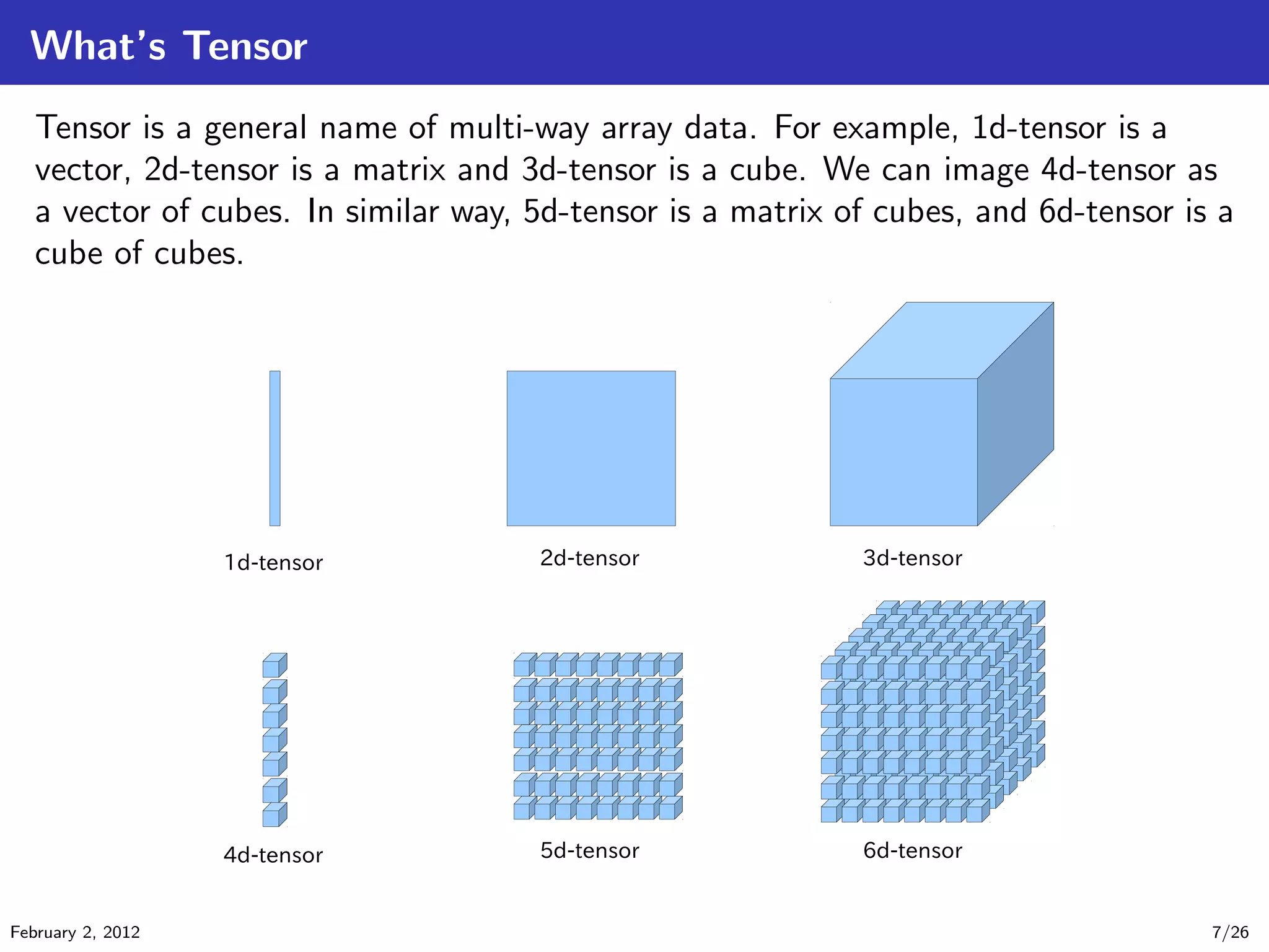
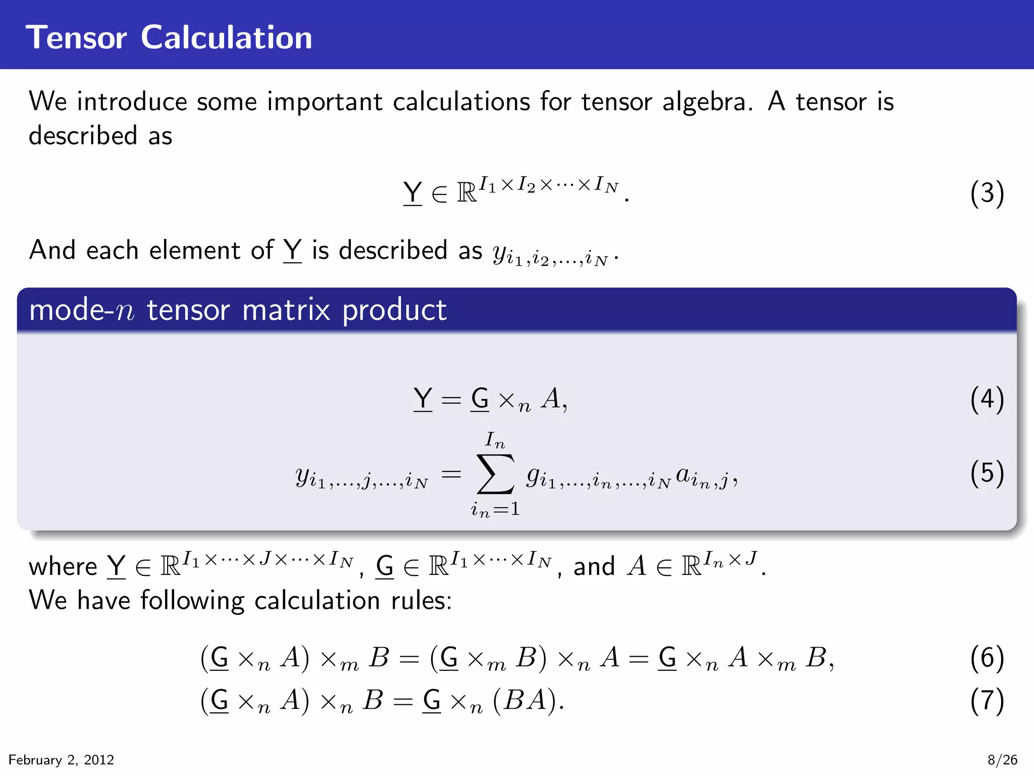
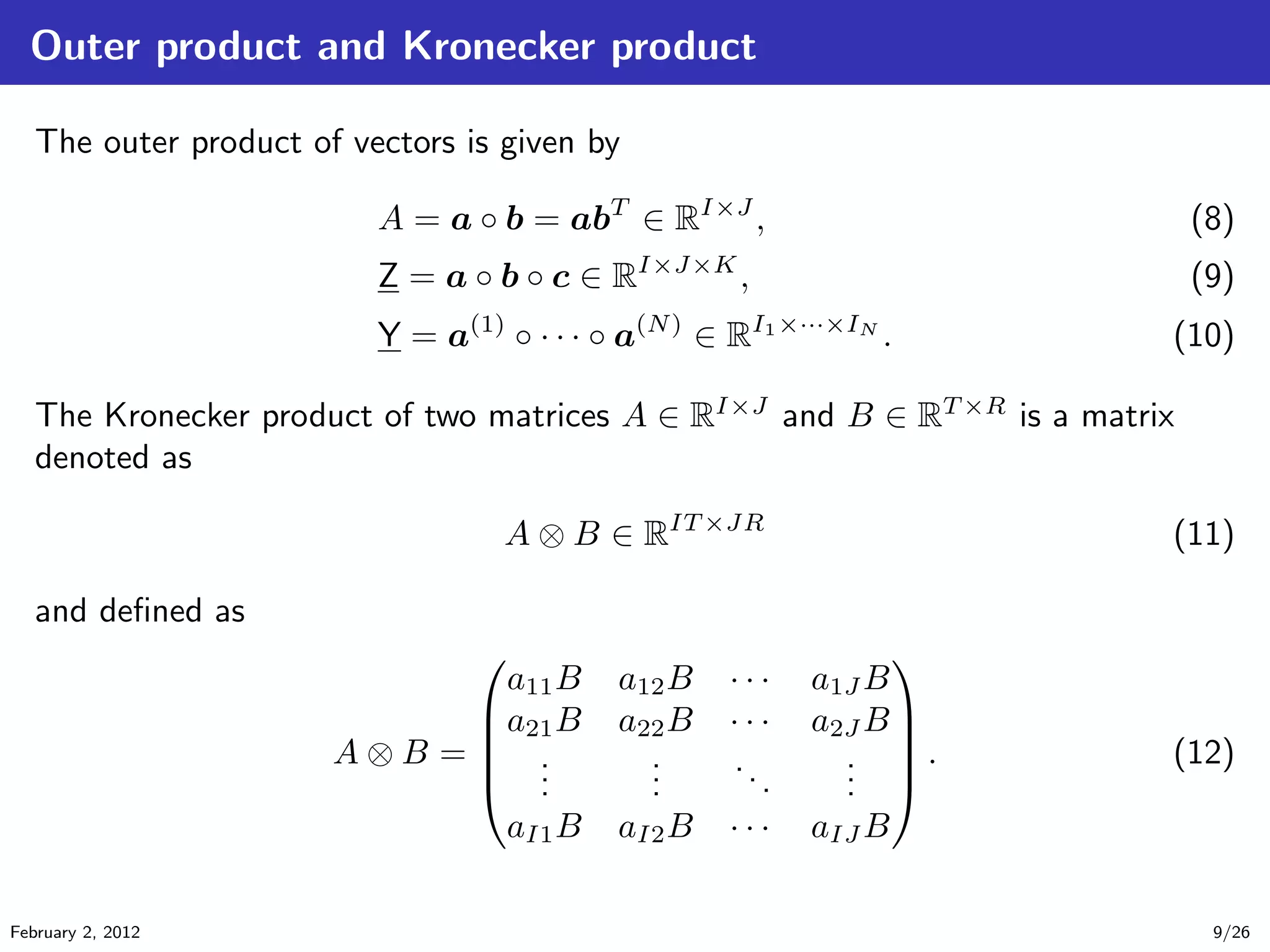
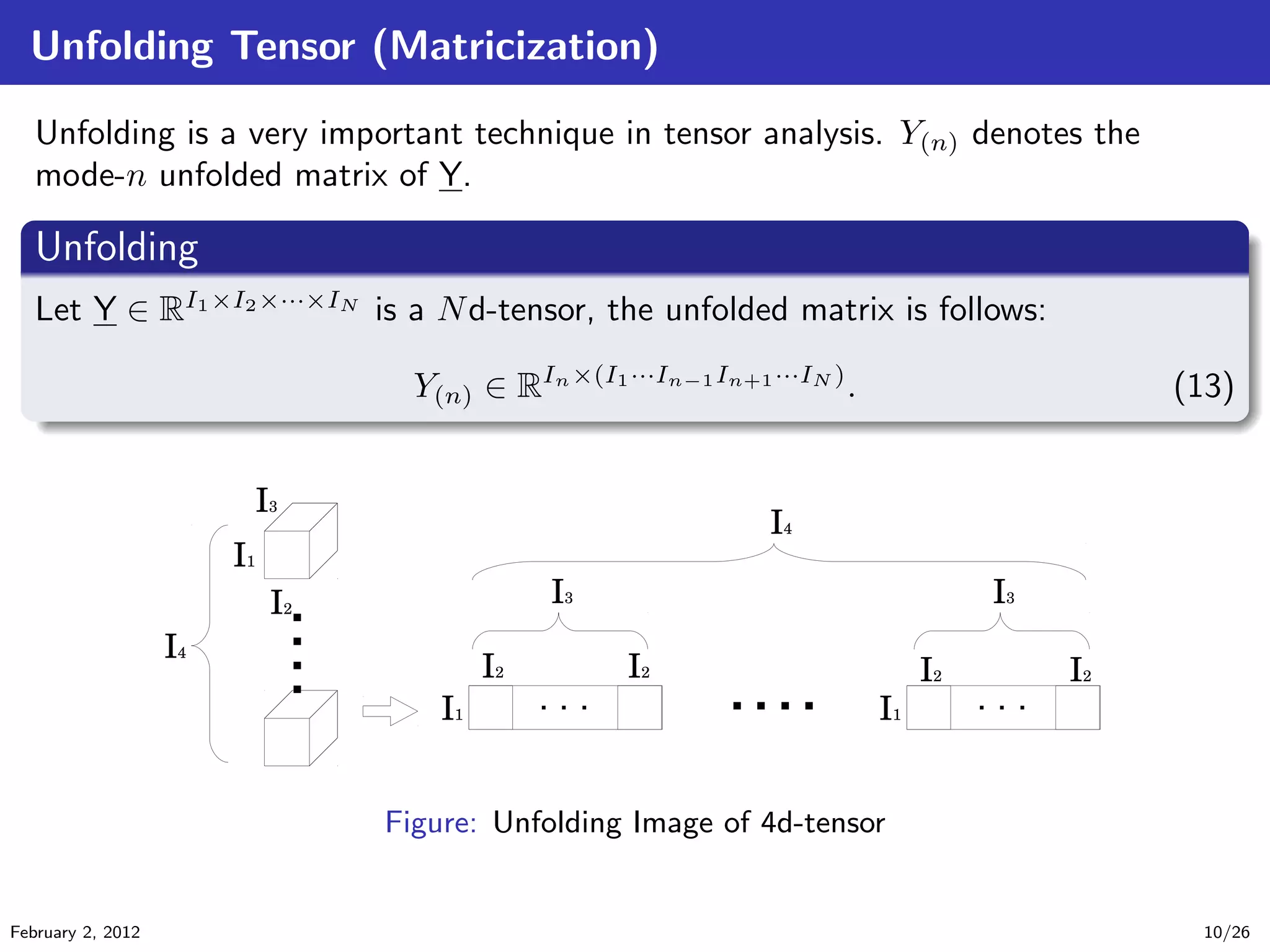
The document details tensor analysis techniques for EEG data in the context of brain-computer interfaces (BCIs), emphasizing the importance of non-invasive methods like EEG due to their low cost and risk. It outlines steps in EEG analysis, introduces tensor calculations and decompositions, and presents experimental results comparing different classification methods. The findings are based on data obtained from a BCI competition involving motor imagery classification.