Why Probability?
• Probabilityrepresents a (standardized)
measure of chance, and quantifies
uncertainty.
• Statistics uses rules of probability as a tool
for making inferences about or describing a
population using data from a sample
3.
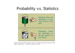
Probability v.s. Statistics
Diagramshowing the difference between statistics and probability. (Image by MIT OpenCourseWare.
Based on Gilbert, Norma. Statistics. W.B. Saunders Co., 1976.)
4.
Sample space andEvents
• Sample space, result of an experiment
Ex: If you toss a coin twice,
• Event A: a subset of
Ex: First toss is head A= {HH,HT}
• S: Event space, a set of events
Ex: {A|A }
5.
Terms
, ,, are called "outcomes" or "sample points"
the elements of are called "sample points"
That's why are called a "sam
, ,
ple sp
,
ace".
HH HT T
HH HT TH T
H TT
o
T
S
6.
Three Probability Axioms
Probabilitysatisfies
• Nonnegativity: for every event A,
• Normalization:
• Additivity: for mutually exclusive events
( ) 0
P A
1
1
( ) ( )
i i
i
i
P A P A
1
P
: | [0,1]
P S A A
i
A
7.
If A isan event, then
P(A) is the probability that
event A occurs.
8.
L. Wang, Departmentof Statistics University of South Carolina; Slide 13
Mutually Exclusive Events
• Mutually exclusive events can not occur
at the same time.
Mutually Exclusive Events Not Mutually
Exclusive Events
9.
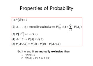
Properties of Probability
Ex:If A and B are mutually exclusive, then
1. P(A∩B)=0
2. P(A∪B) = P ( A )+ P ( B )
1 n
1
1
(1) 0
(2) , , : mutually exclusive ( ) ( )
(3) 1 ( )
(4) ( ) ( )
(5) ( ) ( ) ( ) ( )
n
n
n i
i
i
C
P
A A P A P A
P A P A
A B P A P B
P A B P A P B P A B
10.
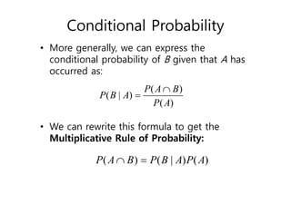
Conditional Probability
• Moregenerally, we can express the
conditional probability of B given that A has
occurred as:
• We can rewrite this formula to get the
Multiplicative Rule of Probability:
( )
( | )
( )
P A B
P B A
P A
( ) ( | ) ( )
P A B P B A P A
11.
Conditional Probability
• Insome cases events are related, so that if we
know event A has occurred then we learn more
about an event B
• Example: Roll a die
A: observe an even number {2,4,6}
B: observe a number less than 4 {1,2,3}
If we know nothing else, then P(B) = 3/6 = 1/2
But if we know A has occurred, then P(B | A) = 1/3
12.
We purchase 30%of our parts from Vendor V.
Vendor V’s defective rate is 5%.
What is the probability that
a randomly chosen part is defective and from Vendor V?
① 0.200
② 0.050
③ 0.015
④ 0.030
L. Wang, Department of Statistics University of South Carolina; Slide 17
P(A)=0.3: We purchase 30% of our parts from Vendor V.
P(B|A)=0.05: Vendor V’s defective rate is 5%.
P(A∩B)=?: What is the probability that
a randomly chosen part is defective and from Vendor V?
[Example of Conditional Probability]
13.
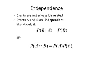
Independence
• Events arenot always be related.
• Events A and B are independent
if and only if:
iff:
( | ) ( )
P B A P B
( ) ( ) ( )
P A B P A P B
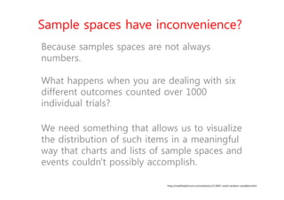
Because samples spacesare not always
numbers.
What happens when you are dealing with six
different outcomes counted over 1000
individual trials?
We need something that allows us to visualize
the distribution of such items in a meaningful
way that charts and lists of sample spaces and
events couldn't possibly accomplish.
http://mathhelpforum.com/statistics/113891-need-random-variables.html
Sample spaces have inconvenience?
16.
Sample spaces haveinconvenience.
So we need something, that are functions
called Random variables.
The term “random” usually means not able to be predicted or happening
by chance. It
17.
Sample spaces haveinconvenience.
So we need something, that are functions
called Random variables.
18.
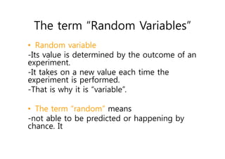
The term “RandomVariables”
• Random variable
-Its value is determined by the outcome of an
experiment.
-It takes on a new value each time the
experiment is performed.
-That is why it is “variable”.
• The term “random” means
-not able to be predicted or happening by
chance. It
19.
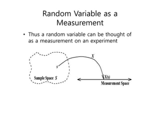
Random Variable asa
Measurement
• Thus a random variable can be thought of
as a measurement on an experiment
X
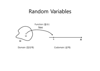
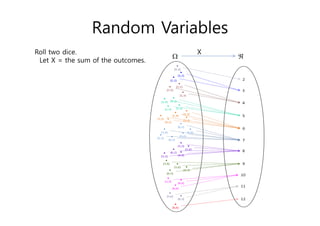
Roll twodice.
Let X = the sum of the outcomes.
Random Variables
22.
Examples of RandomVariables
• Roll two dice.
Let X = number of sixes.
– Possible values of X = {0, 1, 2}.
• Select a player on the LotteGiants.
Let X = his batting average.
– Possible values of X are
{x | 0 ≤ x ≤ 1}.
23.
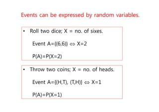
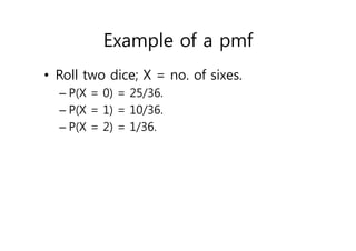
• Roll twodice; X = no. of sixes.
Event A={(6,6)} X=2
P(A)=P(X=2)
• Throw two coins; X = no. of heads.
Event A={(H,T), (T,H)} X=1
P(A)=P(X=1)
Events can be expressed by random variables.
24.
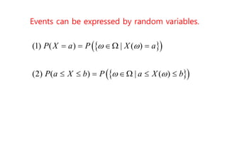
(1) ( ) | ( )
(2) ( ) | ( )
P X a P X a
P a X b P a X b
Events can be expressed by random variables.
25.
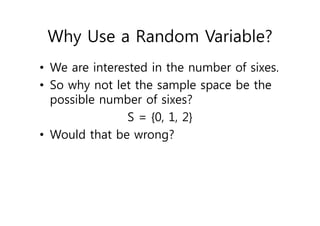
Why Use aRandom Variable?
• We are interested in the number of sixes.
• So why not let the sample space be the
possible number of sixes?
S = {0, 1, 2}
• Would that be wrong?
26.
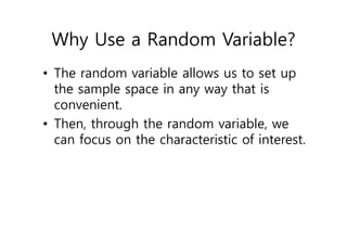
Why Use aRandom Variable?
• The random variable allows us to set up
the sample space in any way that is
convenient.
• Then, through the random variable, we
can focus on the characteristic of interest.
27.
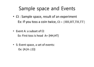
• In manyexperiments, it is easier to deal with a
summary variable than with the original probability
structure.
[Example] In an opinion poll, we ask 50 people whether
agree or disagree with a certain issue.
– Suppose we record a "1" for agree and "0" for disagree.
– The sample space for this experiment has 250 elements.
• Suppose we are only interested in the number of
people who agree.
– Define X=number of "1“ ‘s recorded out of 50.
– Easier to deal with this sample space (has only 51 elements).
CS479/679 Pattern Recognition Spring 2013 – Dr. George Bebis
Why Use a Random Variable?
28.
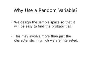
Why Use aRandom Variable?
• We design the sample space so that it
will be easy to find the probabilities.
• This may involve more than just the
characteristic in which we are interested.
29.
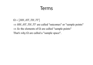
: [0,1]defined as
( )
F R
F x P X x
(Cumulative) Distribution function F of
a random variable X.
30.
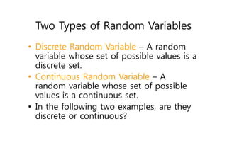
Two Types ofRandom Variables
• Discrete Random Variable – A random
variable whose set of possible values is a
discrete set.
• Continuous Random Variable – A
random variable whose set of possible
values is a continuous set.
• In the following two examples, are they
discrete or continuous?
31.
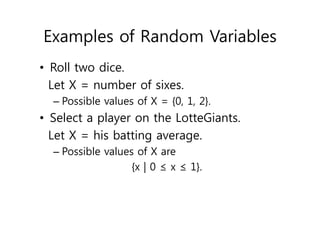
Examples of RandomVariables
• Roll two dice.
Let X = number of sixes.
– Possible values of X = {0, 1, 2}.
• Select a player on the LotteGiants.
Let X = his batting average.
– Possible values of X are
{x | 0 ≤ x ≤ 1}.
32.
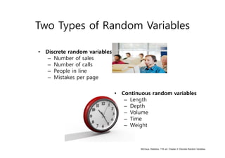
Two Types ofRandom Variables
• Discrete random variables
– Number of sales
– Number of calls
– People in line
– Mistakes per page
• Continuous random variables
– Length
– Depth
– Volume
– Time
– Weight
McClave, Statistics, 11th ed. Chapter 4: Discrete Random Variables
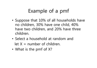
Example of apmf
• Suppose that 10% of all households have
no children, 30% have one child, 40%
have two children, and 20% have three
children.
• Select a household at random and
let X = number of children.
• What is the pmf of X?
38.
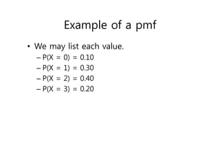
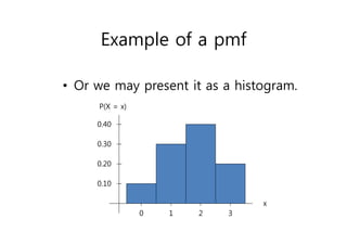
Example of apmf
• We may list each value.
– P(X = 0) = 0.10
– P(X = 1) = 0.30
– P(X = 2) = 0.40
– P(X = 3) = 0.20
39.
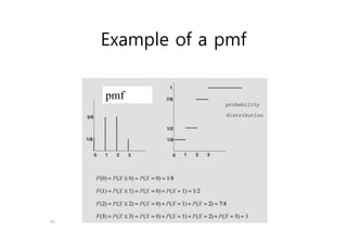
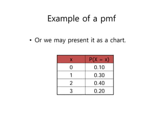
• Or wemay present it as a chart.
x P(X = x)
0 0.10
1 0.30
2 0.40
3 0.20
Example of a pmf
40.
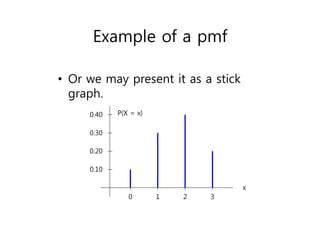
• Or wemay present it as a stick
graph.
x
P(X = x)
0 1 2 3
0.10
0.20
0.30
0.40
Example of a pmf
41.
• Or wemay present it as a histogram.
x
P(X = x)
0 1 2 3
0.10
0.20
0.30
0.40
Example of a pmf
42.
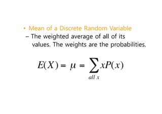
• Mean ofa Discrete Random Variable
– The weighted average of all of its
values. The weights are the probabilities.
43.
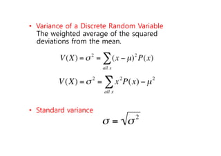
• Variance ofa Discrete Random Variable
The weighted average of the squared
deviations from the mean.
• Standard variance
44.
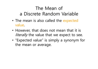
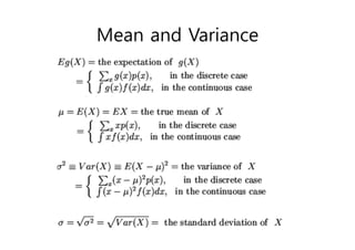
The Mean of
aDiscrete Random Variable
• The mean is also called the expected
value.
• However, that does not mean that it is
literally the value that we expect to see.
• “Expected value” is simply a synonym for
the mean or average.
45.
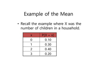
Example of theMean
• Recall the example where X was the
number of children in a household.
x P(X = x)
0 0.10
1 0.30
2 0.40
3 0.20
46.
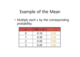
Example of theMean
• Multiply each x by the corresponding
probability.
x P(X = x) xP(X = x)
0 0.10 0.00
1 0.30 0.30
2 0.40 0.80
3 0.20 0.60
47.
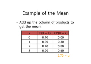
Example of theMean
• Add up the column of products to
get the mean.
x P(X = x) xP(X = x)
0 0.10 0.00
1 0.30 0.30
2 0.40 0.80
3 0.20 0.60
1.70 = µ
48.
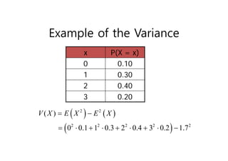
Example of theVariance
x P(X = x)
0 0.10
1 0.30
2 0.40
3 0.20
2 2
2 2 2 2 2
( )
0 0.1 1 0.3 2 0.4 3 0.2 1.7
V X E X E X
49.
Distributions of
discrete randomvariables.
• Discrete Uniform Distribution
• Bernoulli Distribution
• Binomial Distribution
• Geometric Distribution
• …
G. Baker, Departmentof Statistics University of South Carolina; Slide 56
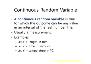
Continuous Random Variable
• A continuous random variable is one
for which the outcome can be any value
in an interval of the real number line.
• Usually a measurement.
• Examples
– Let Y = length in mm
– Let Y = time in seconds
– Let Y = temperature in ºC
52.
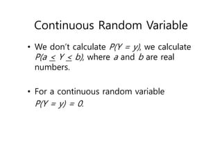
Continuous Random Variable
•We don’t calculate P(Y = y), we calculate
P(a < Y < b), where a and b are real
numbers.
• For a continuous random variable
P(Y = y) = 0.
53.
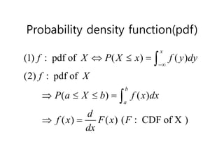
Probability density function(pdf)
(1): pdf of ( ) ( )
(2) : pdf of
( ) ( )
( ) ( ) ( : CDF of X )
x
b
a
f X P X x f y dy
f X
P a X b f x dx
d
f x F x F
dx
54.
Time Spent Waitingfor a Bus
• A bus arrives at a bus stop every 30
minutes. If a person arrives at the bus
stop at a random time, what is the
probability that the person will have to
wait less than 10 minutes for the next
bus?
55.
G. Baker, Departmentof Statistics
University of South Carolina; Slide 60
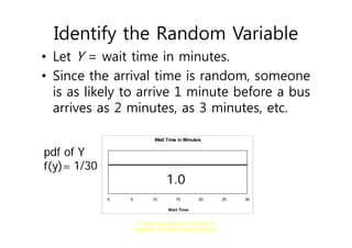
Identify the Random Variable
• Let Y = wait time in minutes.
• Since the arrival time is random, someone
is as likely to arrive 1 minute before a bus
arrives as 2 minutes, as 3 minutes, etc.
Wait Time in Minutes
0 5 10 15 20 25 30
Wait Time
1.0
1/30
pdf of Y
f(y)=
56.
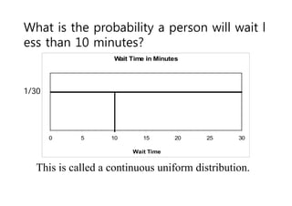
What is theprobability a person will wait l
ess than 10 minutes?
Wait Time in Minutes
0 5 10 15 20 25 30
Wait Time
10/30 = 0.33 20/30 = 0.67
This is called a continuous uniform distribution.
1/30
57.
G. Baker, Departmentof Statistics
University of South Carolina; Slide 62
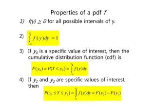
Properties of a pdf f
1) f(y) > 0 for all possible intervals of y.
2)
3) If y0 is a specific value of interest, then the
cumulative distribution function (cdf) is
4) If y1 and y2 are specific values of interest,
then
1
)
( dy
y
f
0
)
(
)
(
)
( 0
0
y
dy
y
f
y
Y
P
y
F
2
1
)
(
)
(
)
(
)
( 1
2
2
1
y
y
y
F
y
F
dy
y
f
y
Y
y
P
58.
G. Baker, Departmentof Statistics
University of South Carolina; Slide 63
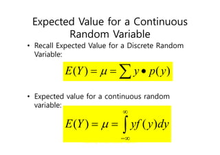
Expected Value for a Continuous
Random Variable
• Recall Expected Value for a Discrete Random
Variable:
• Expected value for a continuous random
variable:
)
(
)
( y
p
y
Y
E
dy
y
yf
Y
E )
(
)
(
59.
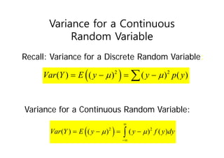
Variance for aContinuous
Random Variable
2 2
( ) ( ) ( ) ( )
Var Y E y y p y
2 2
( ) ( ) ( ) ( )
Var Y E y y f y dy
Recall: Variance for a Discrete Random Variable:
Variance for a Continuous Random Variable:
60.
G. Baker, Departmentof Statistics
University of South Carolina; Slide 65
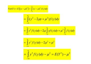
2 2
( ) ( ) ( ) ( )
Var Y E y y f y dy
dy
y
f
y
y )
(
)
2
( 2
2
2
2
2
2
)
(
dy
y
f
y
dy
y
f
dy
y
yf
dy
y
f
y )
(
)
(
2
)
( 2
2
2
2
2
2
)
(
)
(
Y
E
dy
y
f
y
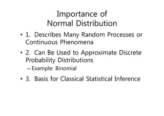
Importance of
Normal Distribution
•1. Describes Many Random Processes or
Continuous Phenomena
• 2. Can Be Used to Approximate Discrete
Probability Distributions
– Example: Binomial
• 3. Basis for Classical Statistical Inference
64.
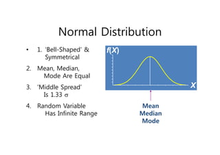
Normal Distribution
• 1.‘Bell-Shaped’ &
Symmetrical
2. Mean, Median,
Mode Are Equal
3. ‘Middle Spread’
Is 1.33
4. Random Variable
Has Infinite Range
Mean
Median
Mode
X
f(X)
X
f(X)
65.
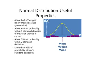
Normal Distribution Useful
Properties
•About half of “weight”
below mean (because
symmetrical)
• About 68% of probability
within 1 standard deviation
of mean (at change in
curve)
• About 95% of probability
within 2 standard
deviations
• More than 99% of
probability within 3
standard deviations
Mean
Median
Mode
X
f(X)
X
f(X)
2
2
3
3
66.
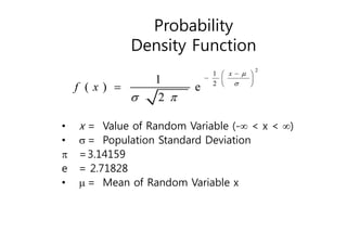
Probability
Density Function
2
1
2
1
( )e
2
x
f x
2
1
2
1
( ) e
2
x
f x
• x = Value of Random Variable (- < x < )
• = Population Standard Deviation
=3.14159
e = 2.71828
• = Mean of Random Variable x
67.
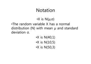
Notation
•X is N(μ,σ)
•Therandom variable X has a normal
distribution (N) with mean μ and standard
deviation σ.
•X is N(40,1)
•X is N(10,5)
•X is N(50,3)
68.
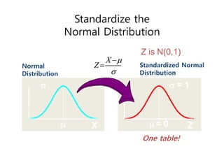
Standardize the
Normal Distribution
X
X
Onetable!
One table!
Normal
Distribution
Normal
Distribution
= 0
= 1
Z
= 0
= 1
Z
X
Z
X
Z
Standardized Normal
Distribution
Standardized Normal
Distribution
Z is N(0,1)
69.
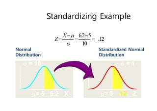
Standardizing Example
X
= 5
= 10
6.2 X
= 5
= 10
6.2
Normal
Distribution
Normal
Distribution
6.2 5
.12
10
X
Z
6.2 5
.12
10
X
Z
Z
= 0
= 1
.12 Z
= 0
= 1
.12
Standardized Normal
Distribution
Standardized Normal
Distribution
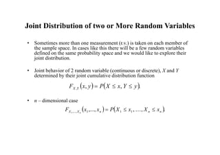
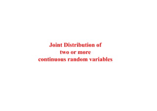
Joint Distribution oftwo or More Random Variables
• Sometimes more than one measurement (r.v.) is taken on each member of
the sample space. In cases like this there will be a few random variables
defined on the same probability space and we would like to explore their
joint distribution.
• Joint behavior of 2 random variable (continuous or discrete), X and Y
determined by their joint cumulative distribution function
• n – dimensional case
.
,
,
, y
Y
x
X
P
y
x
F Y
X
.
,
,
,..., 1
1
1
,...,
1 n
n
n
X
X x
X
x
X
P
x
x
F n
73.
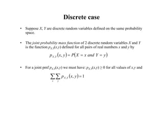
Discrete case
• SupposeX, Y are discrete random variables defined on the same probability
space.
• The joint probability mass function of 2 discrete random variables X and Y
is the function pX,Y(x,y) defined for all pairs of real numbers x and y by
• For a joint pmf pX,Y(x,y) we must have: pX,Y(x,y) ≥ 0 for all values of x,y and
y
Y
and
x
X
P
y
x
p Y
X
,
,
1
,
,
x y
Y
X y
x
p
74.
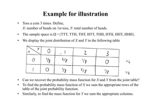
Example for illustration
•Toss a coin 3 times. Define,
X: number of heads on 1st toss, Y: total number of heads.
• The sample space is Ω ={TTT, TTH, THT, HTT, THH, HTH, HHT, HHH}.
• We display the joint distribution of X and Y in the following table
• Can we recover the probability mass function for X and Y from the joint table?
• To find the probability mass function of X we sum the appropriate rows of the
table of the joint probability function.
• Similarly, to find the mass function for Y we sum the appropriate columns.
75.
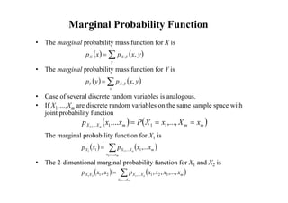
Marginal Probability Function
•The marginal probability mass function for X is
• The marginal probability mass function for Y is
• Case of several discrete random variables is analogous.
• If X1,…,Xm are discrete random variables on the same sample space with
joint probability function
The marginal probability function for X1 is
• The 2-dimentional marginal probability function for X1 and X2 is
y
Y
X
X y
x
p
x
p ,
,
x
Y
X
Y y
x
p
y
p ,
,
m
m
m
X
X x
X
x
X
P
x
x
p n
,...,
,... 1
1
1
,...
1
m
n
x
x
m
X
X
X x
x
p
x
p
,...,
1
,...
1
2
1
1
,...
m
n
x
x
m
X
X
X
X x
x
x
x
p
x
x
p
,...,
3
2
1
,...
2
1
3
1
2
1
,...,
,
,
,
76.
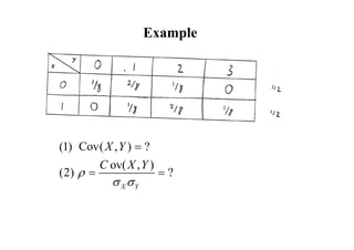
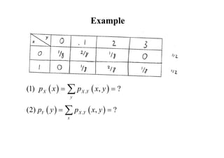
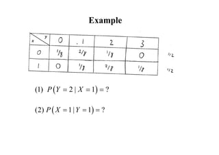
Example
,
(1) , ?
X X Y
y
p x p x y
,
(2) , ?
Y X Y
x
p y p x y
77.
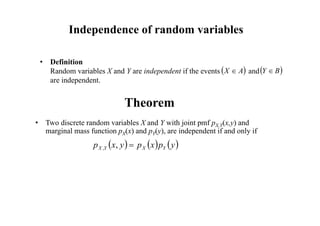
Independence of randomvariables
• Definition
Random variables X and Y are independent if the events and
are independent.
A
X
B
Y
Theorem
• Two discrete random variables X and Y with joint pmf pX,Y(x,y) and
marginal mass function pX(x) and pY(y), are independent if and only if
y
p
x
p
y
x
p Y
X
Y
X
,
,
78.
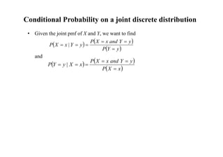
Conditional Probability ona joint discrete distribution
• Given the joint pmf of X and Y, we want to find
and
y
Y
P
y
Y
and
x
X
P
y
Y
x
X
P
|
x
X
P
y
Y
and
x
X
P
x
X
y
Y
P
|
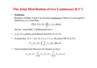
The Joint Distributionof two Continuous R.V’s
• Definition
Random variables X and Y are (jointly) continuous if there is a non-negative
function fX,Y(x,y) such that
for any “reasonable” 2-dimensional set A.
• fX,Y(x,y) is called a joint density function for (X, Y).
• In particular , if A = {(X, Y): X ≤ x, Y ≤ x}, the joint CDF of X,Y is
• From Fundamental Theorem of Calculus we have
A
Y
X dxdy
y
x
f
A
Y
X
P ,
, ,
x y
Y
X
Y
X dv
du
v
u
f
y
x
F ,
,
, ,
,
y
x
F
x
y
y
x
F
y
x
y
x
f Y
X
Y
X
Y
X ,
,
, ,
2
,
2
.
83.
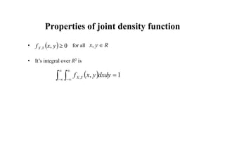
Properties of jointdensity function
• for all
• It’s integral over R2 is
0
,
,
y
x
f Y
X
1
,
, dxdy
y
x
f Y
X
R
y
x
,
84.
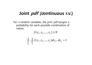
Joint pdf (continuousr.v.)
For n random variables, the joint pdf assigns a
probability for each possible combination of
values:
1 2
( , ,..., ) 0
n
f x x x
1 2 1
... ( , ,..., ) ... 1
n n
R R
f x x x dx dx
85.
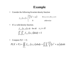
Example
• Consider thefollowing bivariate density function
• It’s a valid density function.
• Compute P(X > Y)
otherwise
y
x
xy
x
y
x
f Y
X
0
1
0
,
1
0
7
12
,
2
,
for all
0
,
,
y
x
f Y
X
1
,
, dxdy
y
x
f Y
X
R
y
x
,
1
2
,
0 0
12
( ) ,
7
x
X Y
x y
P X Y f x y dxdy x xy dydx
86.
week 8 91
Propertiesof Joint Distribution Function
For random variables X, Y , FX,Y : R2 [0,1] given by FX,Y (x,y) = P(X ≤ x,Y ≤ x)
• FX,Y (x,y) is non-decreasing in each variable i.e.
if x1 ≤ x2 and y1 ≤ y2 .
• and
0
,
lim ,
y
x
F Y
X
y
x
1
,
lim ,
y
x
F Y
X
y
x
2
2
,
1
1
, ,
, y
x
F
y
x
F Y
X
Y
X
y
F
y
x
F Y
Y
X
x
,
lim ,
x
F
y
x
F X
Y
X
y
,
lim ,
87.
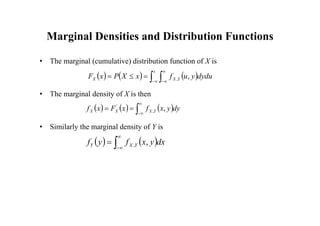
Marginal Densities andDistribution Functions
• The marginal (cumulative) distribution function of X is
• The marginal density of X is then
• Similarly the marginal density of Y is
x
Y
X
X dydu
y
u
f
x
X
P
x
F ,
,
dy
y
x
f
x
F
x
f Y
X
X
X ,
,
'
dx
y
x
f
y
f Y
X
Y ,
,
88.
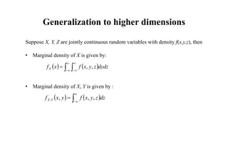
Generalization to higherdimensions
Suppose X, Y, Z are jointly continuous random variables with density f(x,y,z), then
• Marginal density of X is given by:
• Marginal density of X, Y is given by :
dydz
z
y
x
f
x
fX ,
,
dz
z
y
x
f
y
x
f Y
X ,
,
,
,
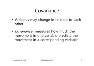
Covariance
• Variables maychange in relation to each
other
• Covariance measures how much the
movement in one variable predicts the
movement in a corresponding variable
95
R F Riesenfeld Sp 2010 CS5961 Comp Stat
91.
Definition of Covariance
Cov(X,Y)= E[(X-X)(Y – Y)]
Alternative Formula
Cov (X,Y)= E(XY) – E(X)E(Y)
Variance of a Sum
Var (X+Y)= Var (X) + Var (Y)+2 Cov (X,Y)
Claim: Covariance is Bilinear
x y
Cov aX b cY d E aX E aX cY E cY
E ac X Y
acCov X Y
( , ) [( ( ))( ( ))]
[ ( )( )]
( , ).
92.
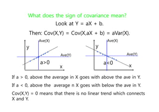
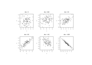
What does thesign of covariance mean?
Look at Y = aX + b.
Then: Cov(X,Y) = Cov(X,aX + b) = aVar(X).
If a > 0, above the average in X goes with above the ave in Y.
If a < 0, above the average n X goes with below the ave in Y.
Cov(X,Y) = 0 means that there is no linear trend which connects
X and Y.
x
y
x
y
a>0 a<0
Ave(Y)
Ave(Y)
Ave(X) Ave(X)
93.
Meaning of thevalue of Covariance
Let HI be height in inches and HC be the height in
centimeters.
Cov(HC,W) = Cov(2.54 HI,W) = 2.54 Cov (HI,W).
So the value depends on the units and is
not very informative!
94.
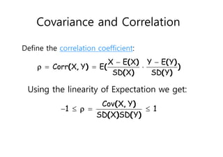
Covariance and Correlation
Definethe correlation coefficient:
X E X Y E Y
Corr X Y E
SD X SD Y
( ) ( )
( , ) ( )
( ) ( )
Cov X Y
1 1
SD X SD Y
( , )
( ) ( )
Using the linearity of Expectation we get:
95.
Covariance and Correlation
Noticethat (aX+b, cY+d) = (X,Y)(a,b>0).
This new quantity is
independent of the change in scale .
So it’s value is quite informative.
96.
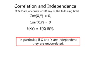
Correlation and Independence
X& Y are uncorrelated iff any of the following hold
Cov(X,Y) = 0,
Corr(X,Y) = 0
E(XY) = E(X) E(Y).
In particular, if X and Y are independent
they are uncorrelated.

![Three Probability Axioms
Probability satisfies
• Nonnegativity: for every event A,
• Normalization:
• Additivity: for mutually exclusive events
( ) 0
P A
1
1
( ) ( )
i i
i
i
P A P A
1
P
: | [0,1]
P S A A
i
A](https://image.slidesharecdn.com/baigiangchapter6-probability-250418080104-b8650d99/85/Bai-giang-Chapter-6-avandce-math-for-engeneering-6-320.jpg)

![We purchase 30% of our parts from Vendor V.
Vendor V’s defective rate is 5%.
What is the probability that
a randomly chosen part is defective and from Vendor V?
① 0.200
② 0.050
③ 0.015
④ 0.030
L. Wang, Department of Statistics University of South Carolina; Slide 17
P(A)=0.3: We purchase 30% of our parts from Vendor V.
P(B|A)=0.05: Vendor V’s defective rate is 5%.
P(A∩B)=?: What is the probability that
a randomly chosen part is defective and from Vendor V?
[Example of Conditional Probability]](https://image.slidesharecdn.com/baigiangchapter6-probability-250418080104-b8650d99/85/Bai-giang-Chapter-6-avandce-math-for-engeneering-12-320.jpg)


![• In many experiments, it is easier to deal with a
summary variable than with the original probability
structure.
[Example] In an opinion poll, we ask 50 people whether
agree or disagree with a certain issue.
– Suppose we record a "1" for agree and "0" for disagree.
– The sample space for this experiment has 250 elements.
• Suppose we are only interested in the number of
people who agree.
– Define X=number of "1“ ‘s recorded out of 50.
– Easier to deal with this sample space (has only 51 elements).
CS479/679 Pattern Recognition Spring 2013 – Dr. George Bebis
Why Use a Random Variable?](https://image.slidesharecdn.com/baigiangchapter6-probability-250418080104-b8650d99/85/Bai-giang-Chapter-6-avandce-math-for-engeneering-27-320.jpg)
![
: [0,1] defined as
( )
F R
F x P X x
(Cumulative) Distribution function F of
a random variable X.](https://image.slidesharecdn.com/baigiangchapter6-probability-250418080104-b8650d99/85/Bai-giang-Chapter-6-avandce-math-for-engeneering-29-320.jpg)

![week 8 91
Properties of Joint Distribution Function
For random variables X, Y , FX,Y : R2 [0,1] given by FX,Y (x,y) = P(X ≤ x,Y ≤ x)
• FX,Y (x,y) is non-decreasing in each variable i.e.
if x1 ≤ x2 and y1 ≤ y2 .
• and
0
,
lim ,
y
x
F Y
X
y
x
1
,
lim ,
y
x
F Y
X
y
x
2
2
,
1
1
, ,
, y
x
F
y
x
F Y
X
Y
X
y
F
y
x
F Y
Y
X
x
,
lim ,
x
F
y
x
F X
Y
X
y
,
lim ,](https://image.slidesharecdn.com/baigiangchapter6-probability-250418080104-b8650d99/85/Bai-giang-Chapter-6-avandce-math-for-engeneering-86-320.jpg)
![Definition of Covariance
Cov (X,Y)= E[(X-X)(Y – Y)]
Alternative Formula
Cov (X,Y)= E(XY) – E(X)E(Y)
Variance of a Sum
Var (X+Y)= Var (X) + Var (Y)+2 Cov (X,Y)
Claim: Covariance is Bilinear
x y
Cov aX b cY d E aX E aX cY E cY
E ac X Y
acCov X Y
( , ) [( ( ))( ( ))]
[ ( )( )]
( , ).
](https://image.slidesharecdn.com/baigiangchapter6-probability-250418080104-b8650d99/85/Bai-giang-Chapter-6-avandce-math-for-engeneering-91-320.jpg)