Order Picking include Pick Sequencing and Batching

1. Order Picking:
Pick Sequencing and Batching

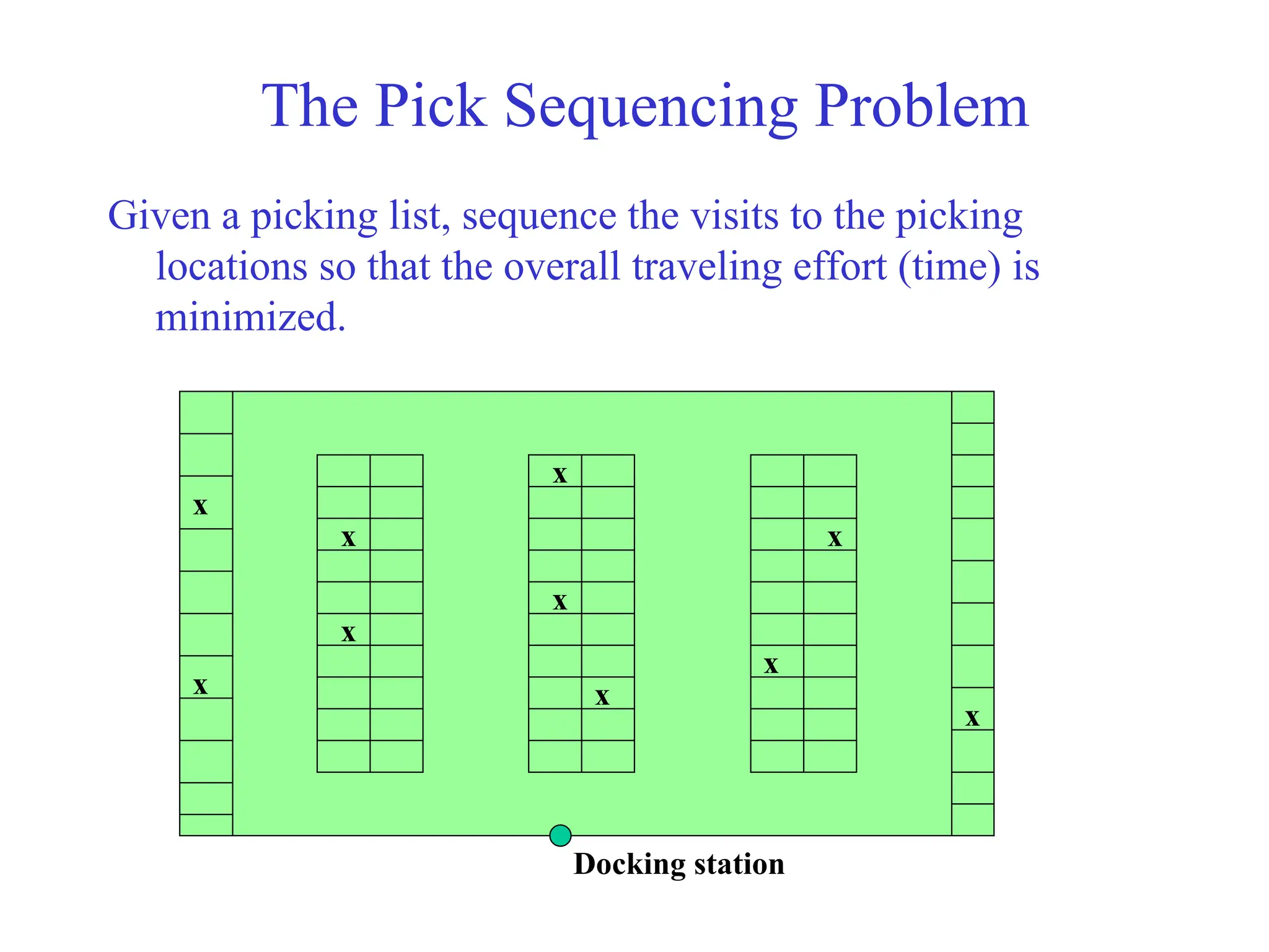
2. The Pick Sequencing Problem
Given a picking list, sequence the visits to the picking
locations so that the overall traveling effort (time) is
minimized.
x
x
x
x
x
x
x
x
x
x
Docking station

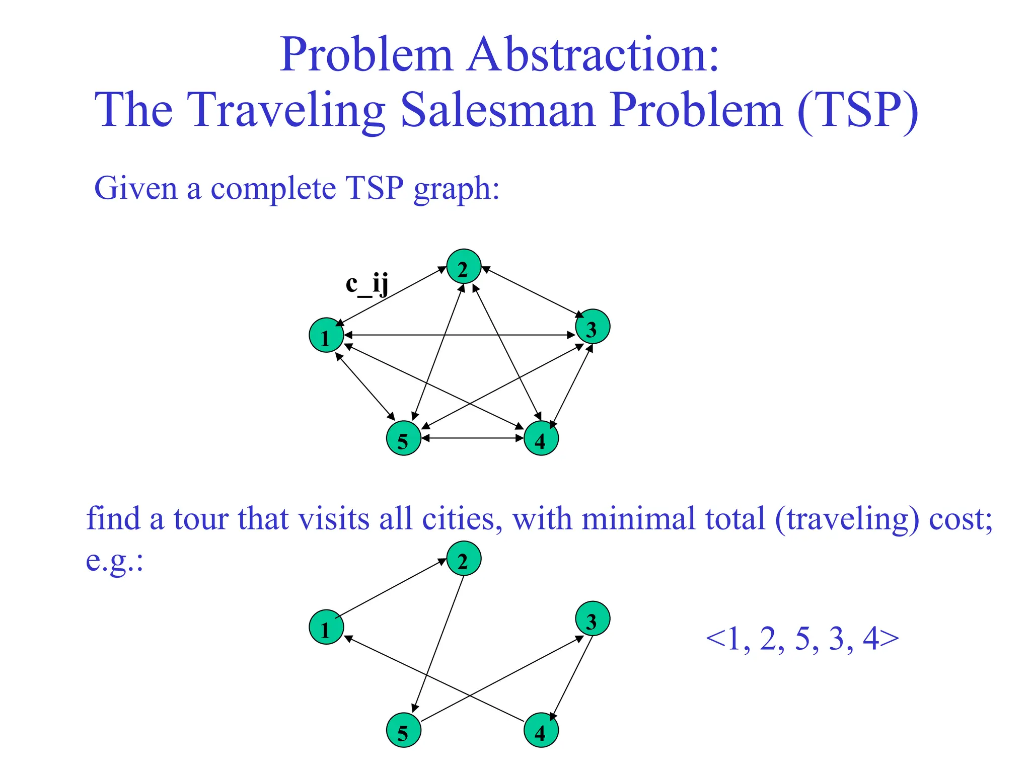
3. Problem Abstraction:
The Traveling Salesman Problem (TSP)
Given a complete TSP graph:
1
2
3
4
5
c_ij
find a tour that visits all cities, with minimal total (traveling) cost;
e.g.:
1
2
3
4
5
<1, 2, 5, 3, 4>

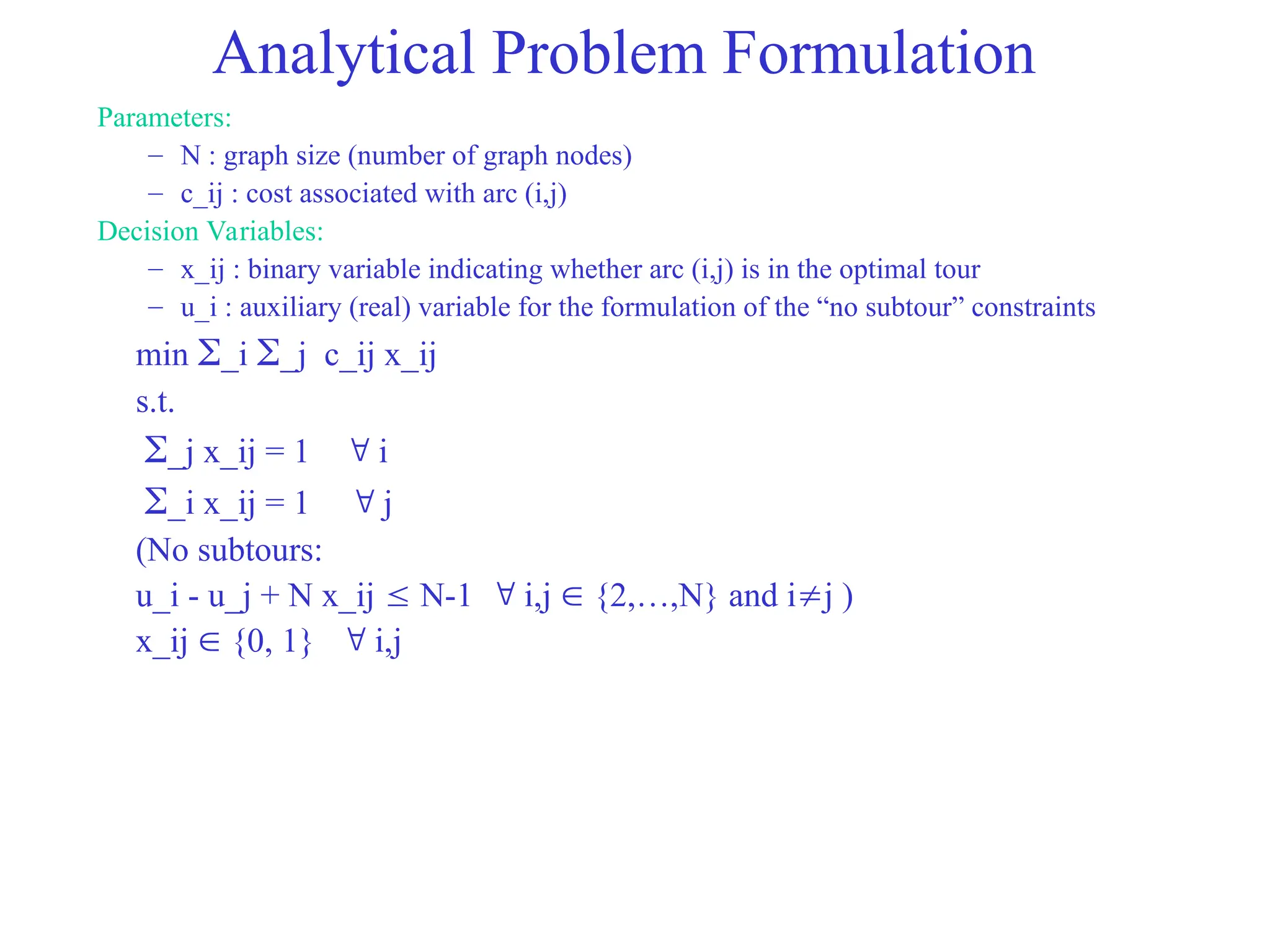
4. Analytical Problem Formulation
Parameters:
– N : graph size (number of graph nodes)
– c_ij : cost associated with arc (i,j)
Decision Variables:
– x_ij : binary variable indicating whether arc (i,j) is in the optimal tour
– u_i : auxiliary (real) variable for the formulation of the “no subtour” constraints
min _i _j c_ij x_ij
s.t.
_j x_ij = 1  i
_i x_ij = 1  j
(No subtours:
u_i - u_j + N x_ij  N-1  i,j  {2,…,N} and ij )
x_ij  {0, 1}  i,j

5. Some remarks on the TSP problem and
its application in pick sequencing
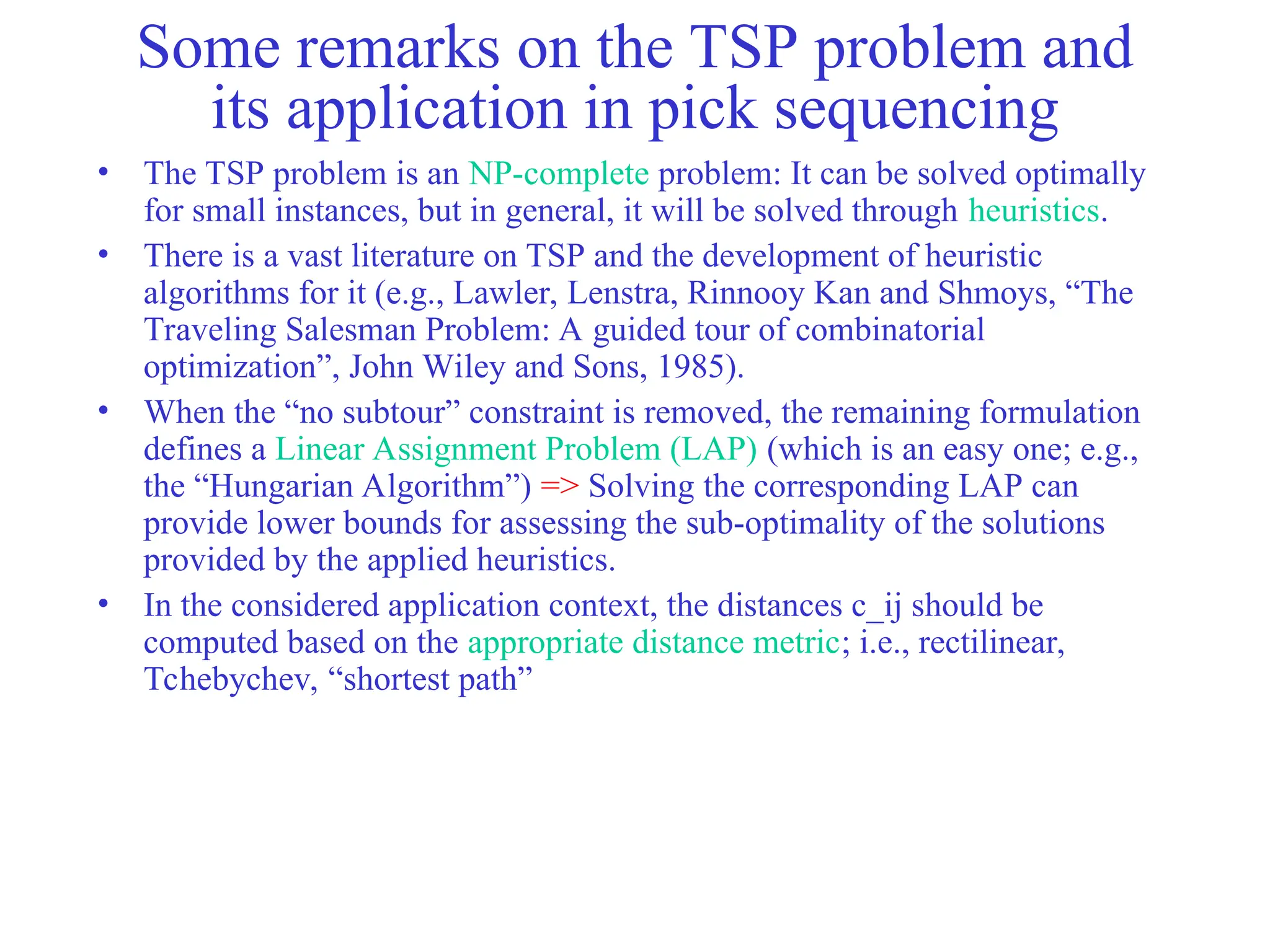
• The TSP problem is an NP-complete problem: It can be solved optimally
for small instances, but in general, it will be solved through heuristics.
• There is a vast literature on TSP and the development of heuristic
algorithms for it (e.g., Lawler, Lenstra, Rinnooy Kan and Shmoys, “The
Traveling Salesman Problem: A guided tour of combinatorial
optimization”, John Wiley and Sons, 1985).
• When the “no subtour” constraint is removed, the remaining formulation
defines a Linear Assignment Problem (LAP) (which is an easy one; e.g.,
the “Hungarian Algorithm”) => Solving the corresponding LAP can
provide lower bounds for assessing the sub-optimality of the solutions
provided by the applied heuristics.
• In the considered application context, the distances c_ij should be
computed based on the appropriate distance metric; i.e., rectilinear,
Tchebychev, “shortest path”

6. The closest insertion algorithm:
A TSP heuristic (symmetric version)
Initialization:
S_p = <1>; S_a = {2,…,N}; c(j) = 1,  j  {2,…,N}; n=1;
While n < N do
n = n+1;
Selection step:
j* = argmin_{j  S_a} {c_{j,c(j)}};
S_a = S_a {j*};
Insertion step:
i* = argmin_{i =1}^|S_p| {c_{[i],j*} + c_{j*,[i mod |S_p|+1]}
- c_{[i],[i mod |S_p|+1]}};
S_p = < [1],…,[i*], j*, [i*+1],…,[n]>;
 j  S_a, if c_{j,j*} < c_{j,c(j)} then c(j) = j*;
Remarks: 1. [i] denotes the node at i-th position of the constructed sub-tour.
2. If the distances are symmetric and satisfy the triangular inequality, the cost of the solution provided by this heuristic is no
worse than twice the optimal cost.

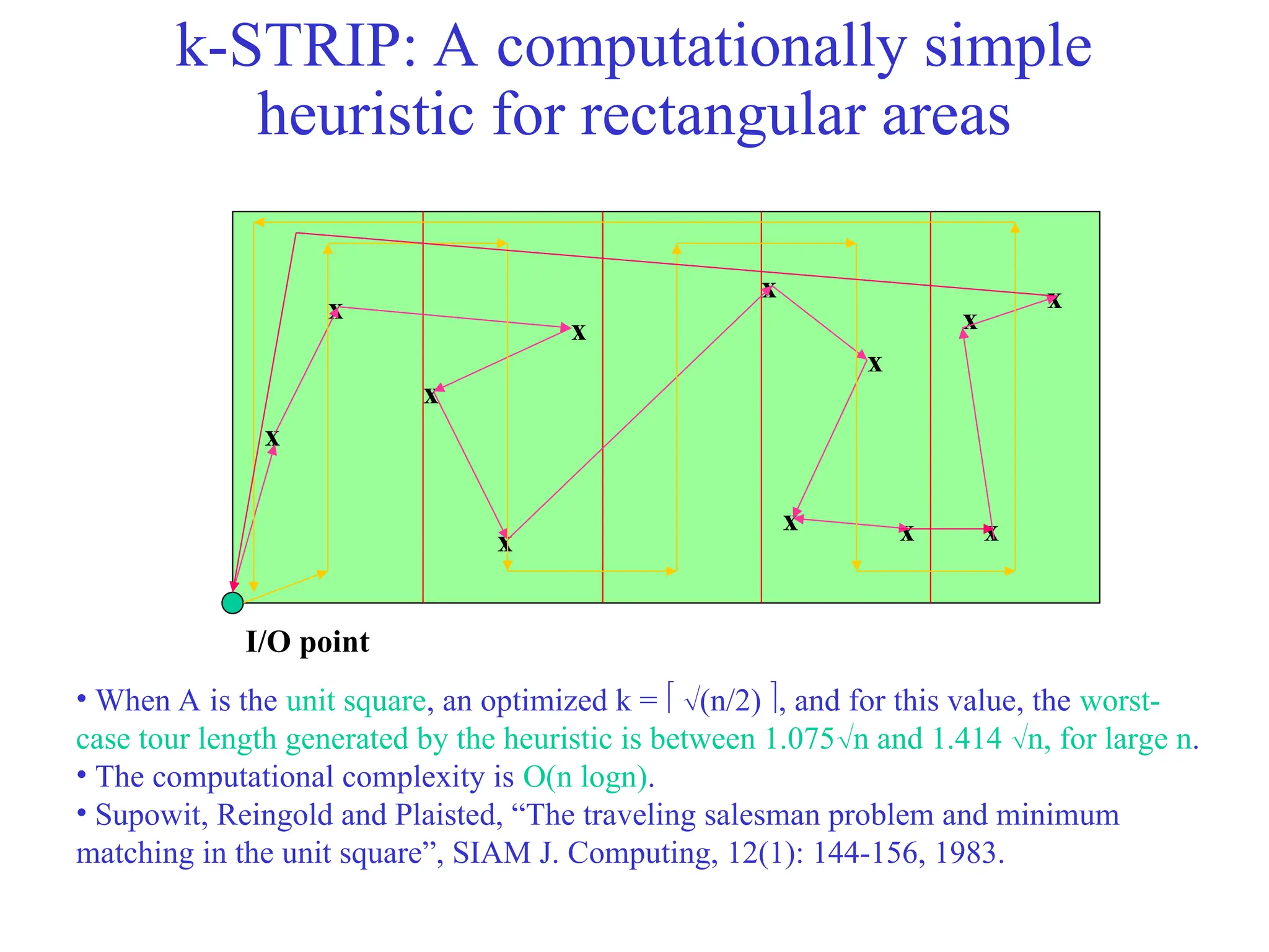
7. k-STRIP: A computationally simple
heuristic for rectangular areas
x
x
x
x
x
x
x
x
x
x
I/O point
x
x
• When A is the unit square, an optimized k =  (n/2) , and for this value, the worst-
case tour length generated by the heuristic is between 1.075n and 1.414 n, for large n.
• The computational complexity is O(n logn).
• Supowit, Reingold and Plaisted, “The traveling salesman problem and minimum
matching in the unit square”, SIAM J. Computing, 12(1): 144-156, 1983.

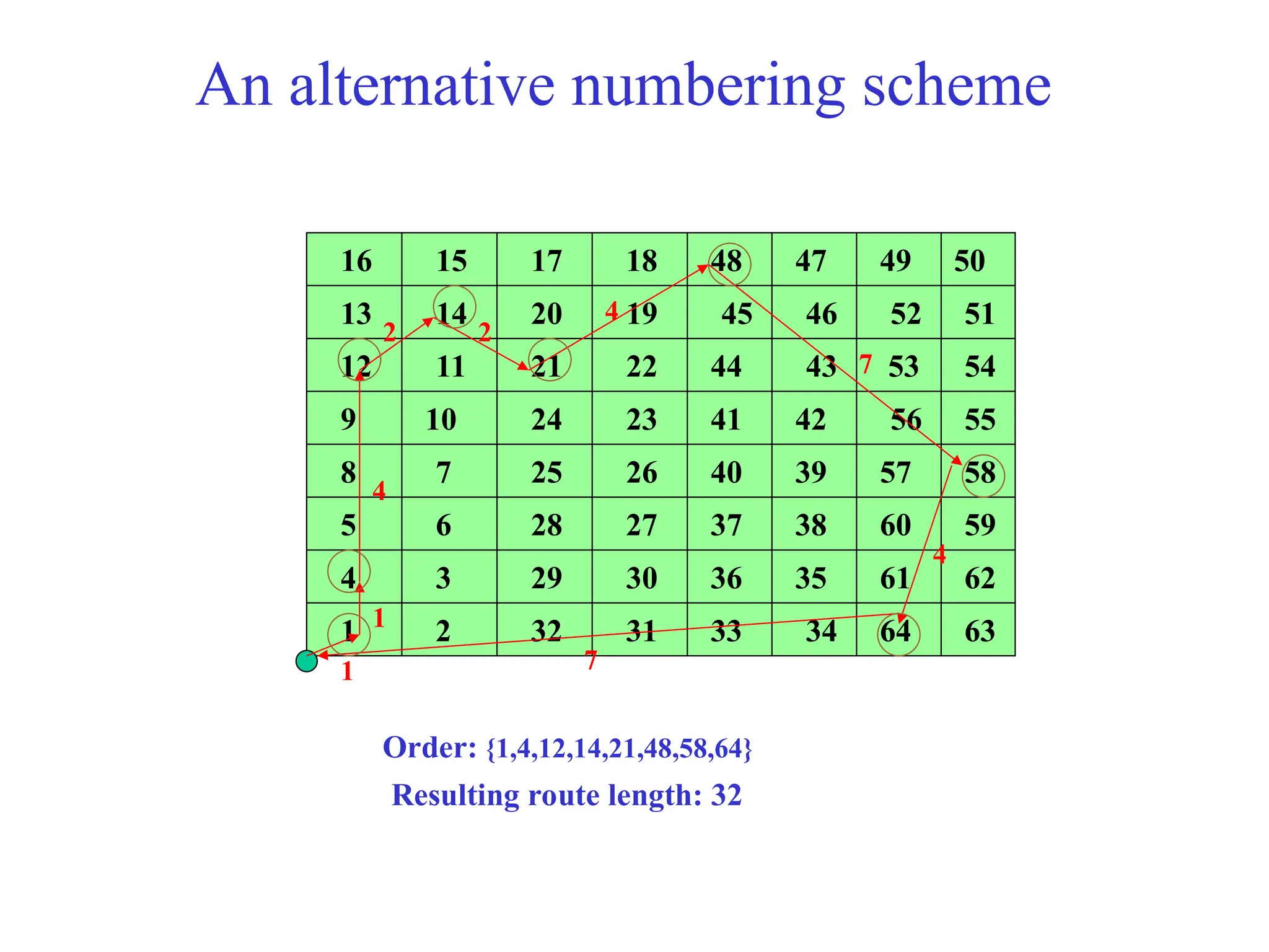
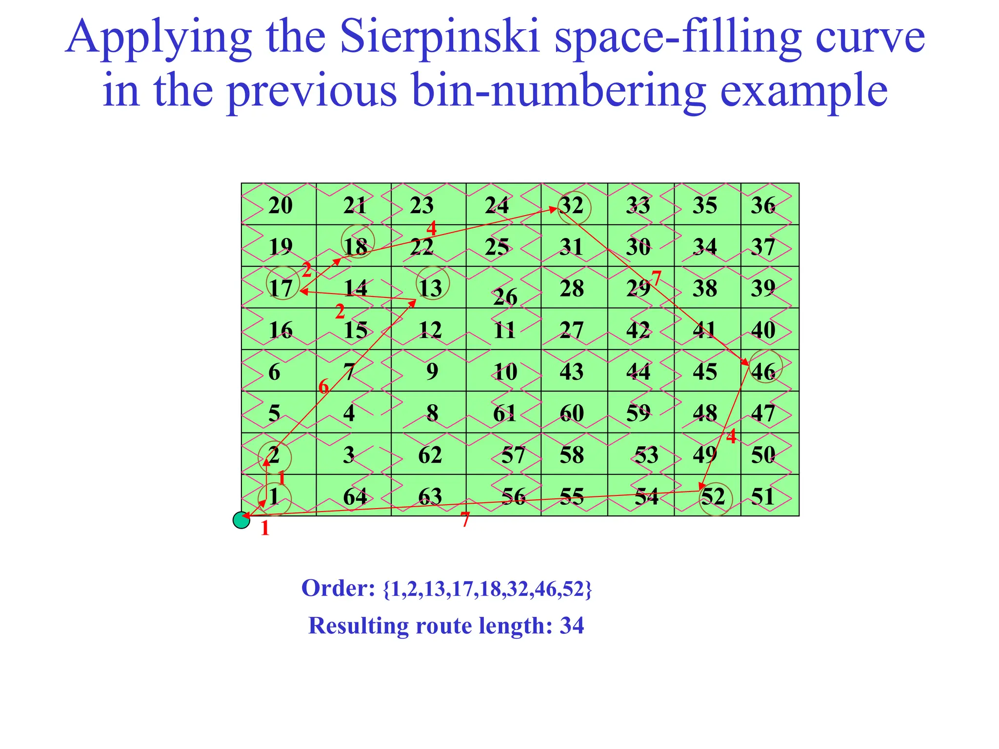
8. The bin-numbering heuristic
(Bartholdi and Platzman, Material Flow, 4: 247-254, 1988)
• Basic idea: Number bins / storage locations in a way that
filling the orders by visiting the associated bins in
increasing numbers will lead to efficient routings.
• Advantages:
– Once the numbering is established, developing the order routes
becomes extremely simple.
– Easy to adjust routes dynamically upon the arrival of new orders.
• Basic underlying problem:
How do you establish good bin-numbering schemes?

9. Example of a numbering scheme
(Is it a good one?)
Order: {1, 10, 13, 28, 30, 44, 50, 62}
1
2
3
4
5
6
7
8
9 10
11
12
13
14
15
16 17
18
19
20 21 22
23
24
25 26
27
28
29
30
31
32 33 34
35
36 37
38
39
40
41
42
43
64
44
45
46
47
48
49
50 51 52
53
54 55
56
57
58
59
60
61
62
63
1 6
7
4
2 2
4
7
11
Resulting route length: 44 (using rectilinear distances of the cell
centroids)

10. An alternative numbering scheme
1 2
3
4
5 6
7
8
9 10
11
12
13
15
16 17 18
19
20
21 22
23
24
25 26
27
28
29 30
31
32 33 34
35
36
38
37
40 39
42
41
44
64
43
45 46
47
48 49 50
51
52
53 54
55
56
57 58
59
60
61 62
63
14
Order: {1,4,12,14,21,48,58,64}
1
1
4
2 2
4
7
4
7
Resulting route length: 32

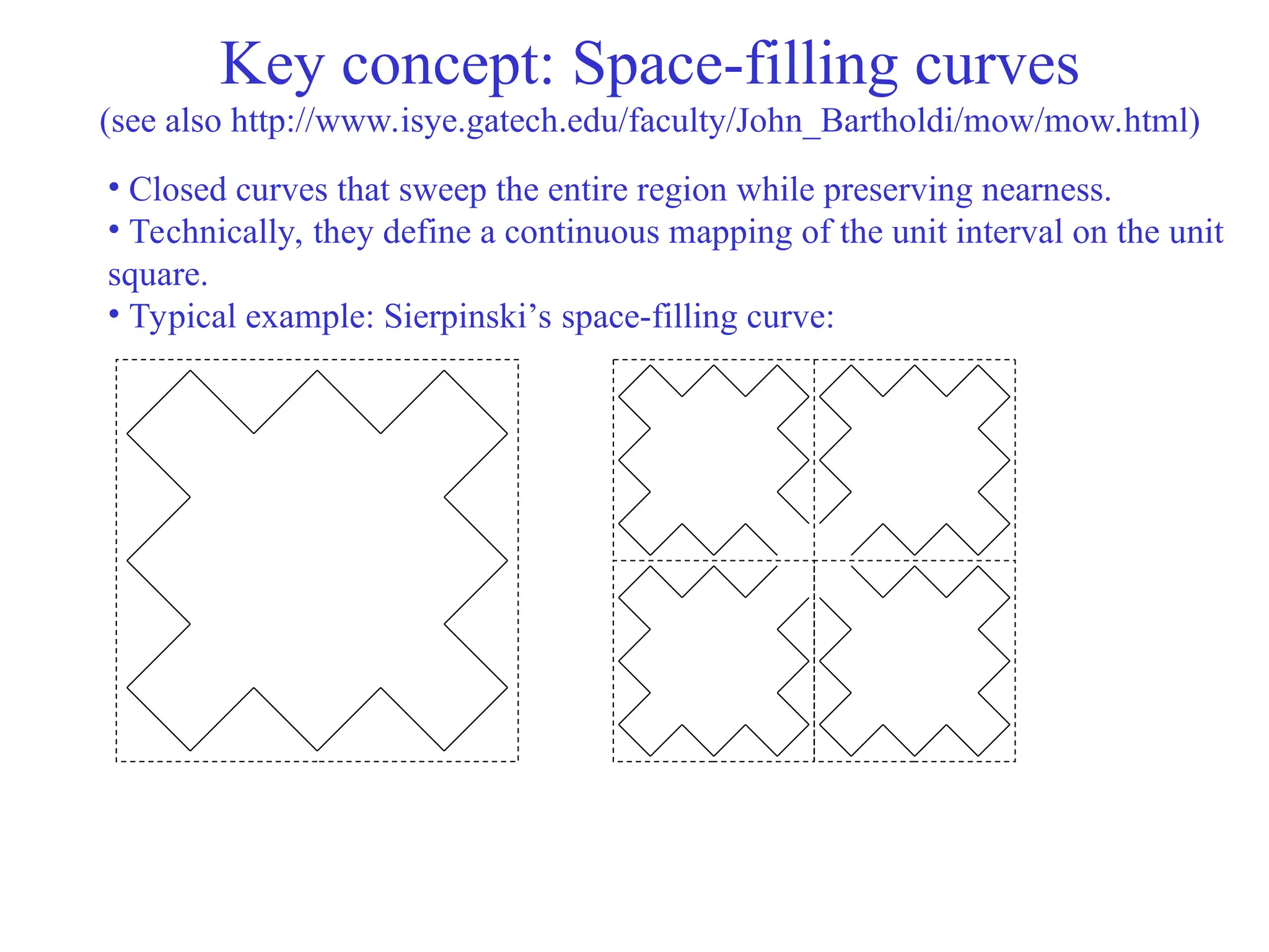
11. Key concept: Space-filling curves
(see also http://www.isye.gatech.edu/faculty/John_Bartholdi/mow/mow.html)
• Closed curves that sweep the entire region while preserving nearness.
• Technically, they define a continuous mapping of the unit interval on the unit
square.
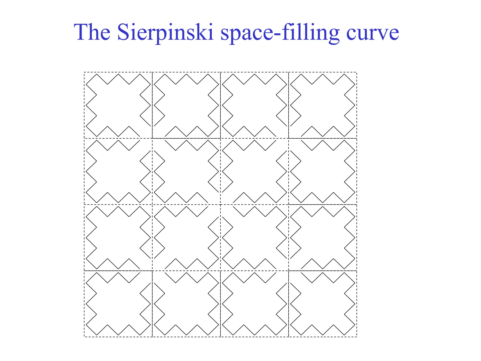
• Typical example: Sierpinski’s space-filling curve:

12. The Sierpinski space-filling curve

13. Applying the Sierpinski space-filling curve
in the previous bin-numbering example
1
2 3
4
5
6 7
8
9 10
11
12
13
15
16
17
18
19
20 21
22
23 24
25
26
27
28 29
30
31
32 33
34
35 36
37
38 39
40
41
42
43
64
44 45 46
47
48
49 50
51
52
53
54
55
56
57 58
59
60
61
62
63
14
Order: {1,2,13,17,18,32,46,52}
Resulting route length: 34
1
1
6
2
2
4
7
4
7

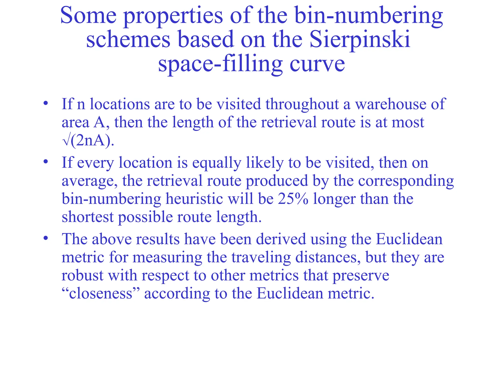
14. Some properties of the bin-numbering
schemes based on the Sierpinski
space-filling curve
• If n locations are to be visited throughout a warehouse of
area A, then the length of the retrieval route is at most
(2nA).
• If every location is equally likely to be visited, then on
average, the retrieval route produced by the corresponding
bin-numbering heuristic will be 25% longer than the
shortest possible route length.
• The above results have been derived using the Euclidean
metric for measuring the traveling distances, but they are
robust with respect to other metrics that preserve
“closeness” according to the Euclidean metric.

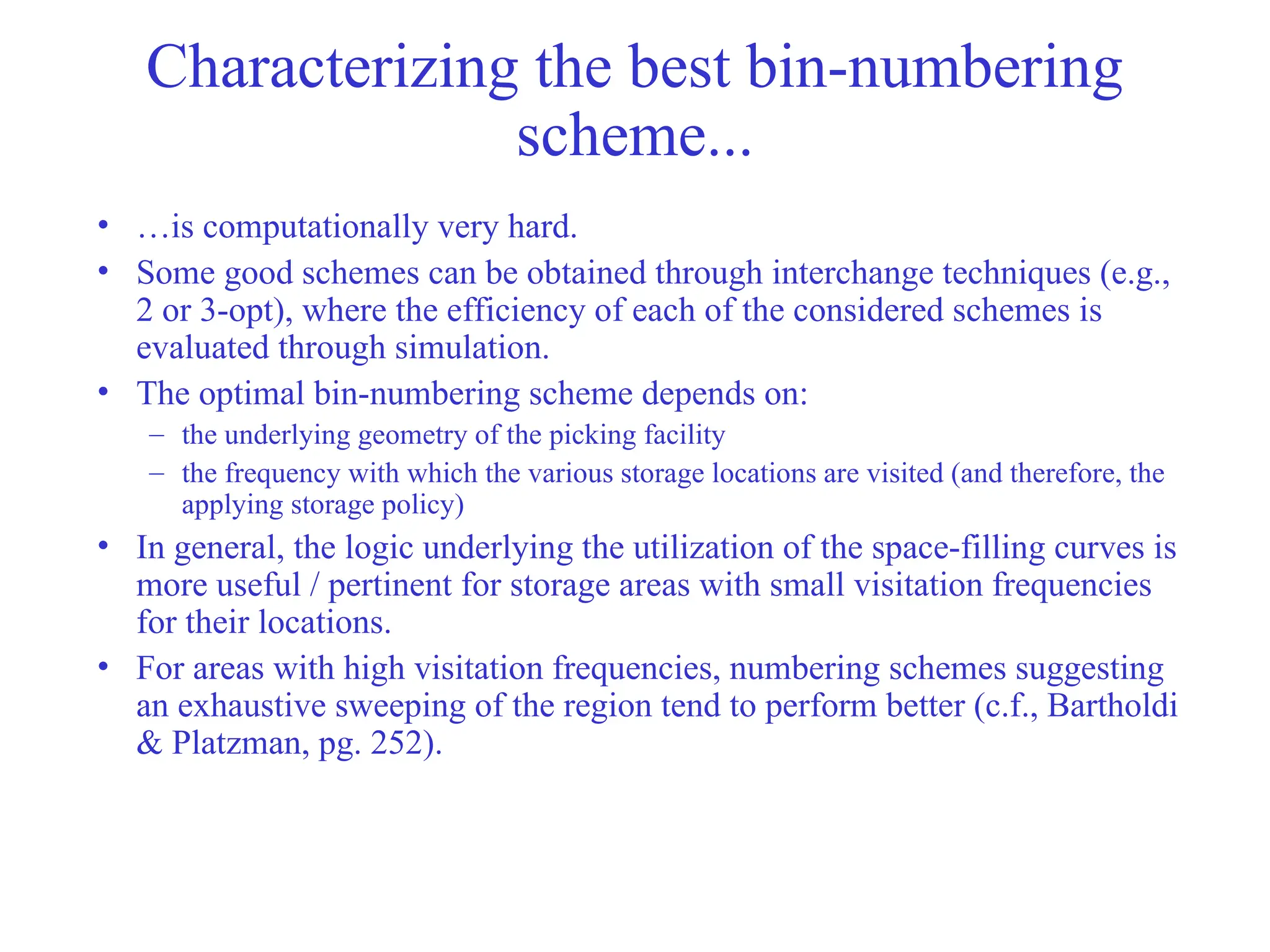
15. Characterizing the best bin-numbering
scheme...
• …is computationally very hard.
• Some good schemes can be obtained through interchange techniques (e.g.,
2 or 3-opt), where the efficiency of each of the considered schemes is
evaluated through simulation.
• The optimal bin-numbering scheme depends on:
– the underlying geometry of the picking facility
– the frequency with which the various storage locations are visited (and therefore, the
applying storage policy)
• In general, the logic underlying the utilization of the space-filling curves is
more useful / pertinent for storage areas with small visitation frequencies
for their locations.
• For areas with high visitation frequencies, numbering schemes suggesting
an exhaustive sweeping of the region tend to perform better (c.f., Bartholdi
& Platzman, pg. 252).

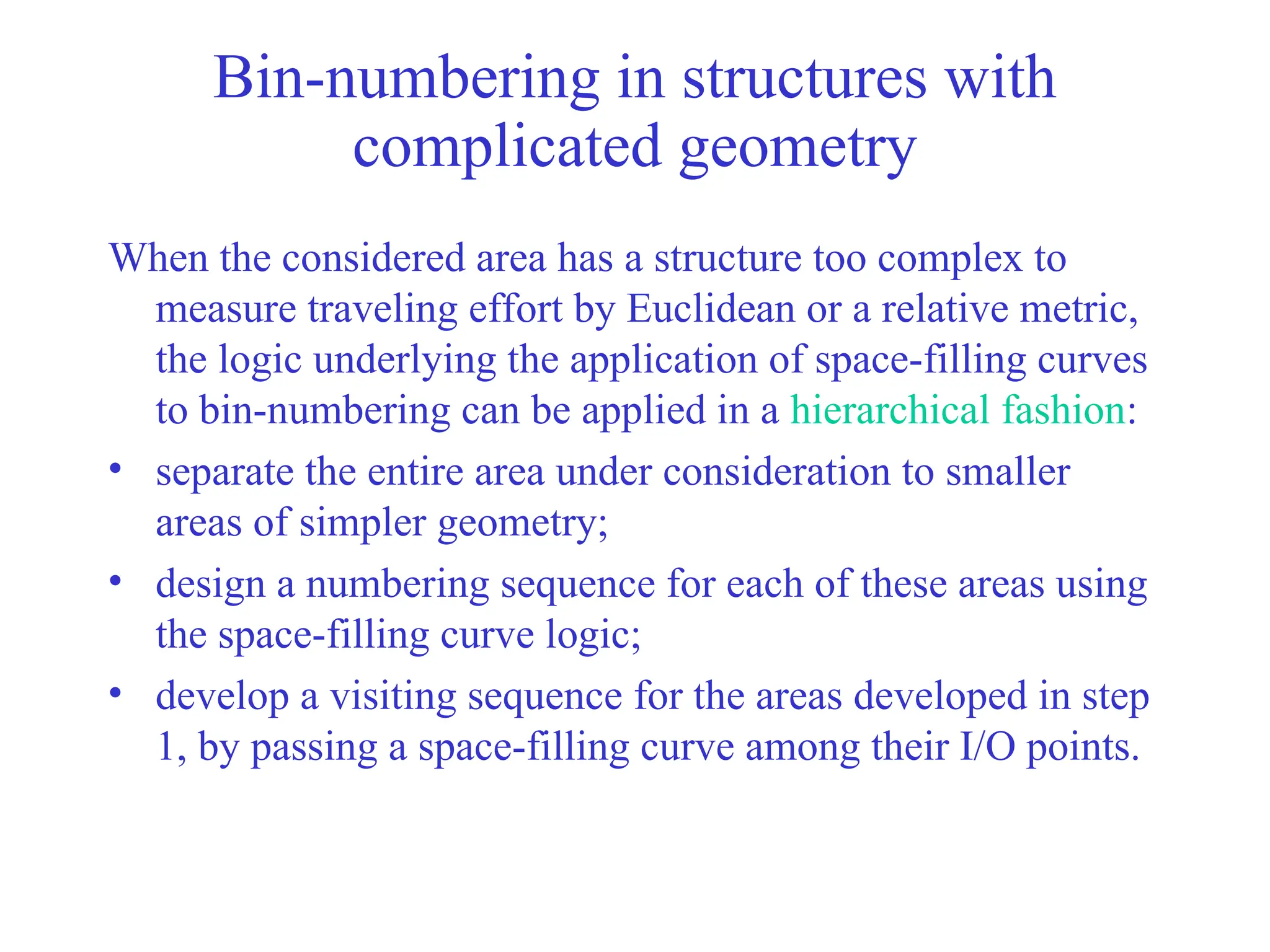
16. Bin-numbering in structures with
complicated geometry
When the considered area has a structure too complex to
measure traveling effort by Euclidean or a relative metric,
the logic underlying the application of space-filling curves
to bin-numbering can be applied in a hierarchical fashion:
• separate the entire area under consideration to smaller
areas of simpler geometry;
• design a numbering sequence for each of these areas using
the space-filling curve logic;
• develop a visiting sequence for the areas developed in step
1, by passing a space-filling curve among their I/O points.

17. Order Batching
(based on De Koster et. al., “Efficient
orderbatching methods in warehouses”, Inlt.
Jrnl of Prod. Res., Vol. 37, No. 7, pgs 1479-
1504, 1999)

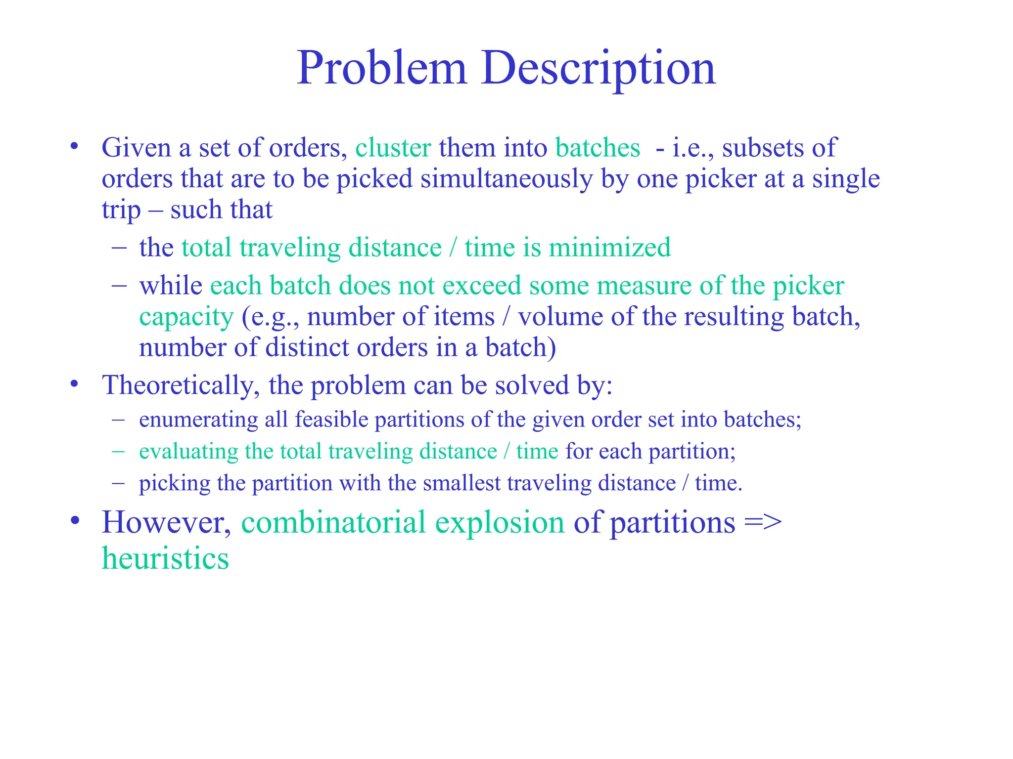
18. Problem Description
• Given a set of orders, cluster them into batches - i.e., subsets of
orders that are to be picked simultaneously by one picker at a single
trip – such that
– the total traveling distance / time is minimized
– while each batch does not exceed some measure of the picker
capacity (e.g., number of items / volume of the resulting batch,
number of distinct orders in a batch)
• Theoretically, the problem can be solved by:
– enumerating all feasible partitions of the given order set into batches;
– evaluating the total traveling distance / time for each partition;
– picking the partition with the smallest traveling distance / time.
• However, combinatorial explosion of partitions =>
heuristics

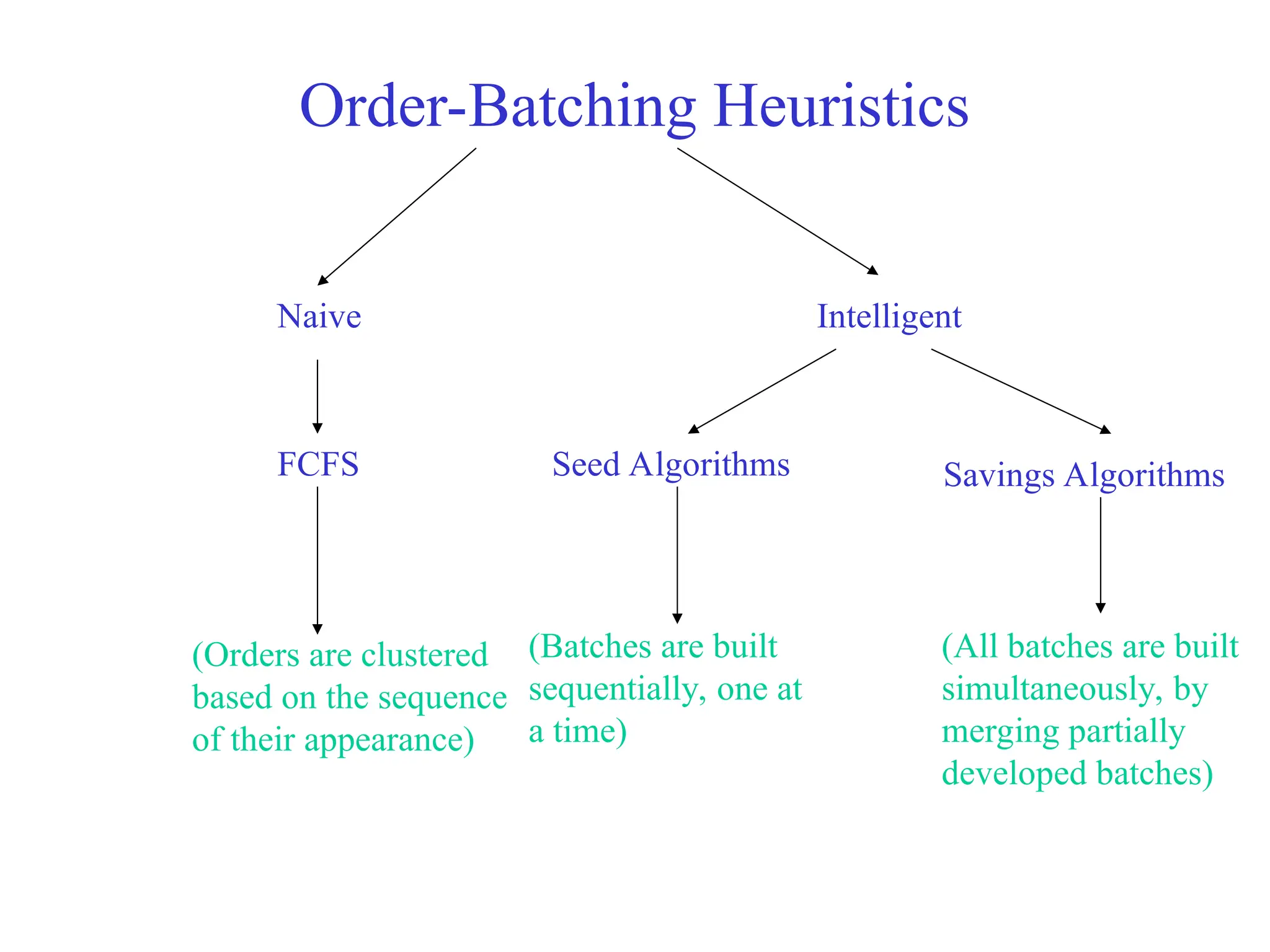
19. Order-Batching Heuristics
Naive Intelligent
FCFS Seed Algorithms Savings Algorithms
(Batches are built
sequentially, one at
a time)
(All batches are built
simultaneously, by
merging partially
developed batches)
(Orders are clustered
based on the sequence
of their appearance)

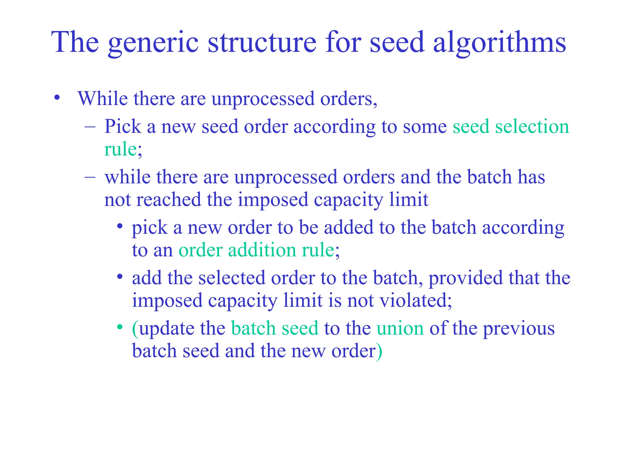
20. The generic structure for seed algorithms
• While there are unprocessed orders,
– Pick a new seed order according to some seed selection
rule;
– while there are unprocessed orders and the batch has
not reached the imposed capacity limit
• pick a new order to be added to the batch according
to an order addition rule;
• add the selected order to the batch, provided that the
imposed capacity limit is not violated;
• (update the batch seed to the union of the previous
batch seed and the new order)

21. Typical seed selection rules
• Random selection
• the order with the farthest item (w.r.t. the shipping station)
• the order with the largest number of aisles to be visited
• the order with the largest aisle range (absolute difference between
the most left aisle number and the most right aisle number to be
visited)
• the order with the largest number of items
• the order with the longest travel time
• Remark: If the batch seed is updated after every order addition, the
algorithm is characterized as dynamic or cumulative mode; ow., it
is said to be static or single mode.

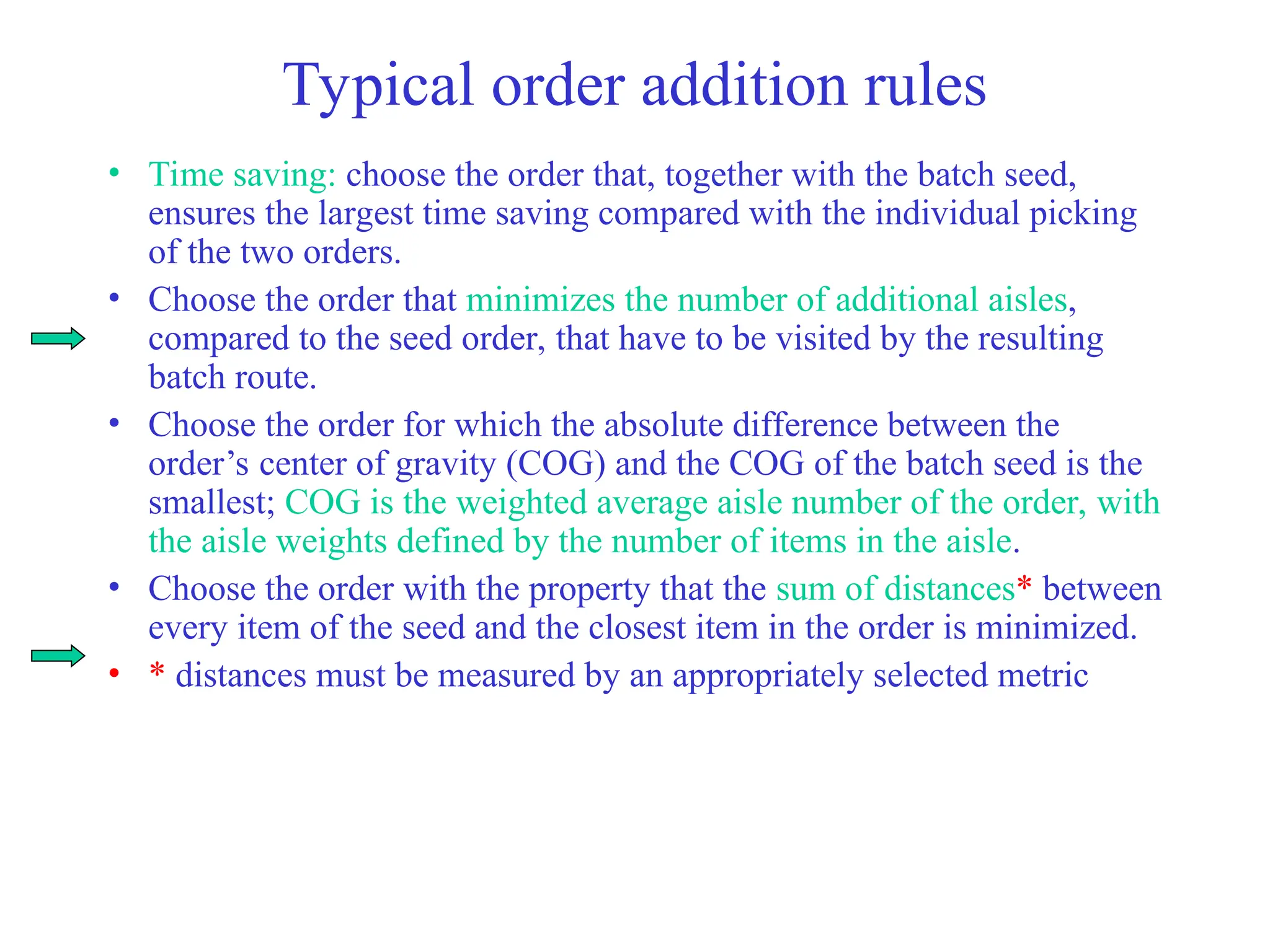
22. Typical order addition rules
• Time saving: choose the order that, together with the batch seed,
ensures the largest time saving compared with the individual picking
of the two orders.
• Choose the order that minimizes the number of additional aisles,
compared to the seed order, that have to be visited by the resulting
batch route.
• Choose the order for which the absolute difference between the
order’s center of gravity (COG) and the COG of the batch seed is the
smallest; COG is the weighted average aisle number of the order, with
the aisle weights defined by the number of items in the aisle.
• Choose the order with the property that the sum of distances* between
every item of the seed and the closest item in the order is minimized.
• * distances must be measured by an appropriately selected metric

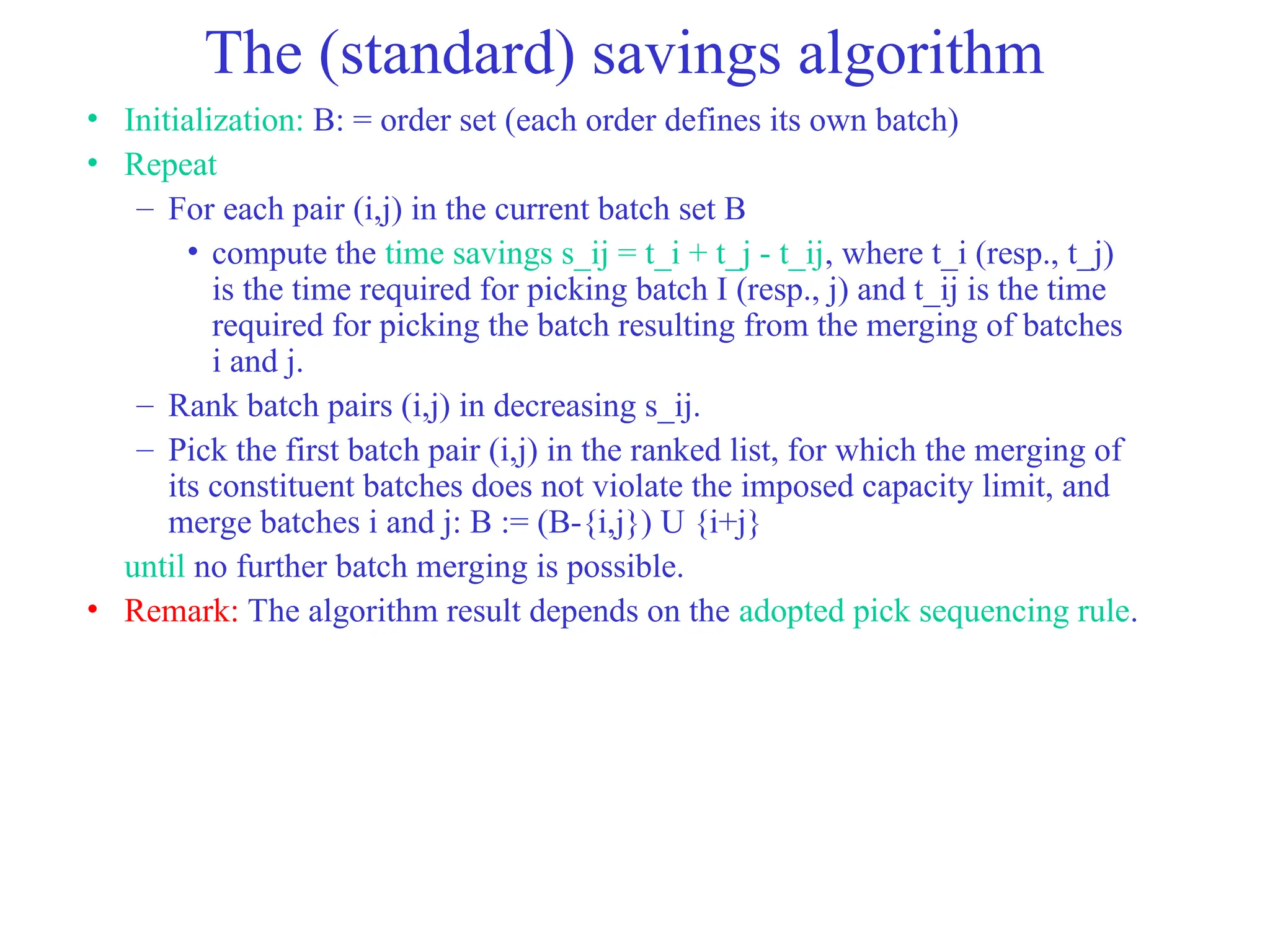
23. The (standard) savings algorithm
• Initialization: B: = order set (each order defines its own batch)
• Repeat
– For each pair (i,j) in the current batch set B
• compute the time savings s_ij = t_i + t_j - t_ij, where t_i (resp., t_j)
is the time required for picking batch I (resp., j) and t_ij is the time
required for picking the batch resulting from the merging of batches
i and j.
– Rank batch pairs (i,j) in decreasing s_ij.
– Pick the first batch pair (i,j) in the ranked list, for which the merging of
its constituent batches does not violate the imposed capacity limit, and
merge batches i and j: B := (B-{i,j}) U {i+j}
until no further batch merging is possible.
• Remark: The algorithm result depends on the adopted pick sequencing rule.

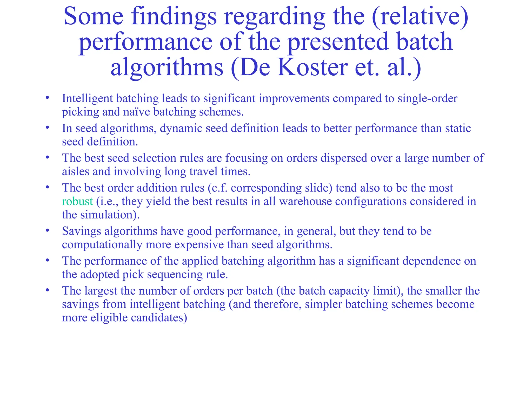
24. Some findings regarding the (relative)
performance of the presented batch
algorithms (De Koster et. al.)
• Intelligent batching leads to significant improvements compared to single-order
picking and naïve batching schemes.
• In seed algorithms, dynamic seed definition leads to better performance than static
seed definition.
• The best seed selection rules are focusing on orders dispersed over a large number of
aisles and involving long travel times.
• The best order addition rules (c.f. corresponding slide) tend also to be the most
robust (i.e., they yield the best results in all warehouse configurations considered in
the simulation).
• Savings algorithms have good performance, in general, but they tend to be
computationally more expensive than seed algorithms.
• The performance of the applied batching algorithm has a significant dependence on
the adopted pick sequencing rule.
• The largest the number of orders per batch (the batch capacity limit), the smaller the
savings from intelligent batching (and therefore, simpler batching schemes become
more eligible candidates)

25. Addendum:
A special case admitting
polynomial solution
(Ratliff and Rosenthal, Operations Research,
31(3): 507-521, 1983)

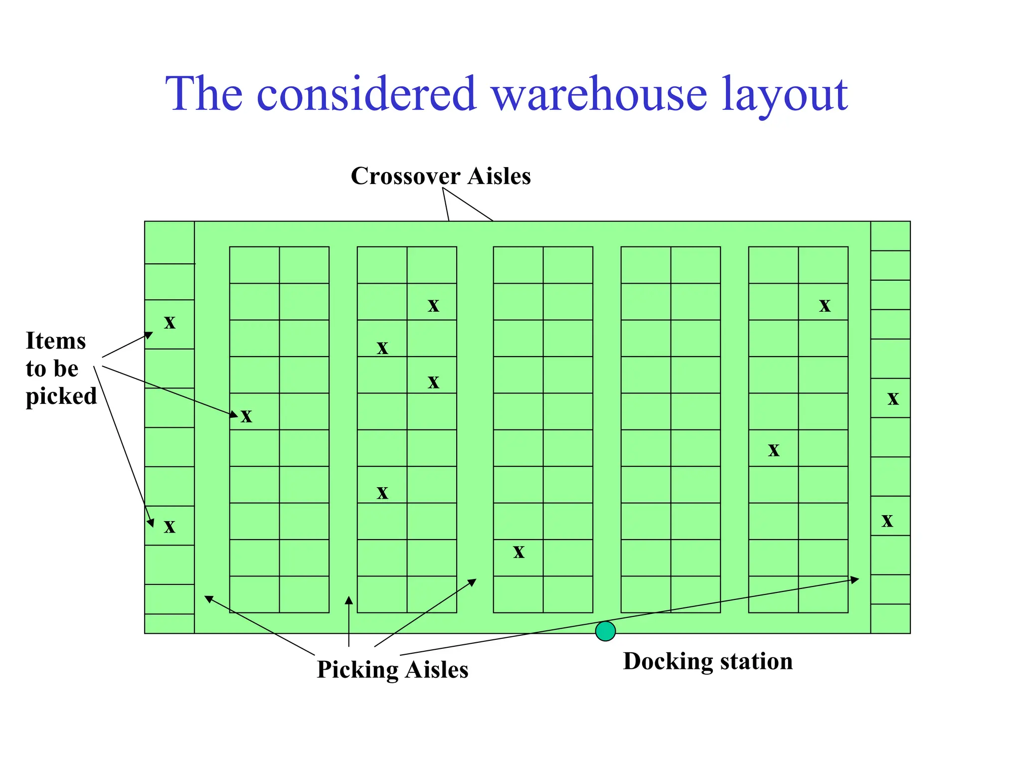
26. The considered warehouse layout
Docking station
Picking Aisles
Crossover Aisles
Items
to be
picked
x
x
x
x
x
x
x
x
x
x
x
x

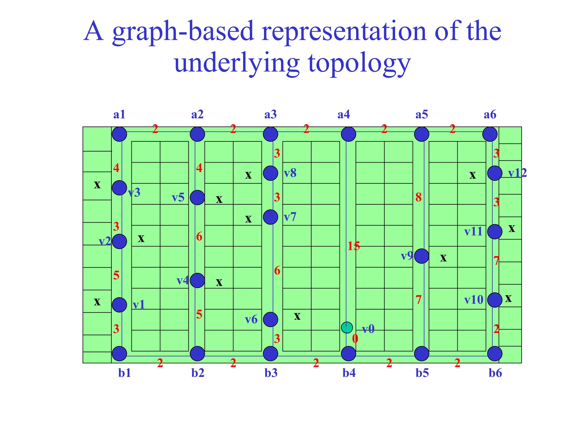
27. A graph-based representation of the
underlying topology
x
x
x
x
x
x
x
x
x
x
x
x
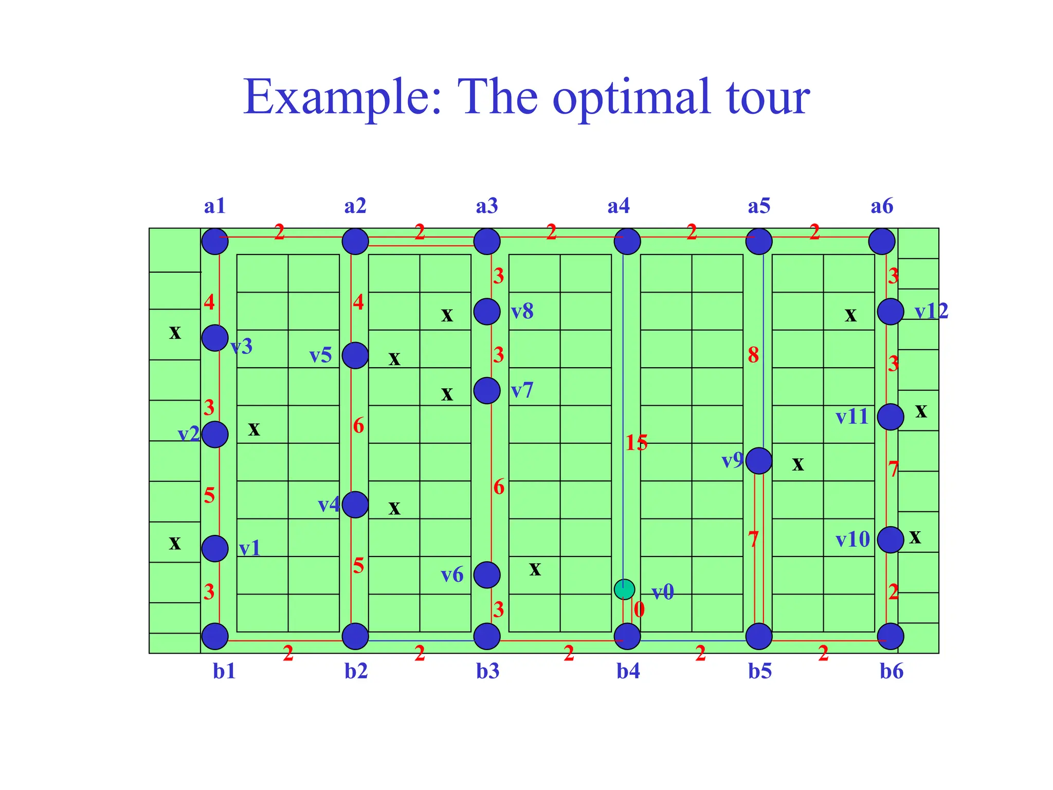
b1 b2 b3 b4 b5 b6
a1 a2 a3 a4 a5 a6
v0
v1
v2
v3
v4
v5
v6
v7
v8
v9
v10
v11
v12
2
2
2 2 2
2
7
3
3
2 2 2
2 2
3
5
3
4 4
6
5
3
6
3
3
15
8
7
0

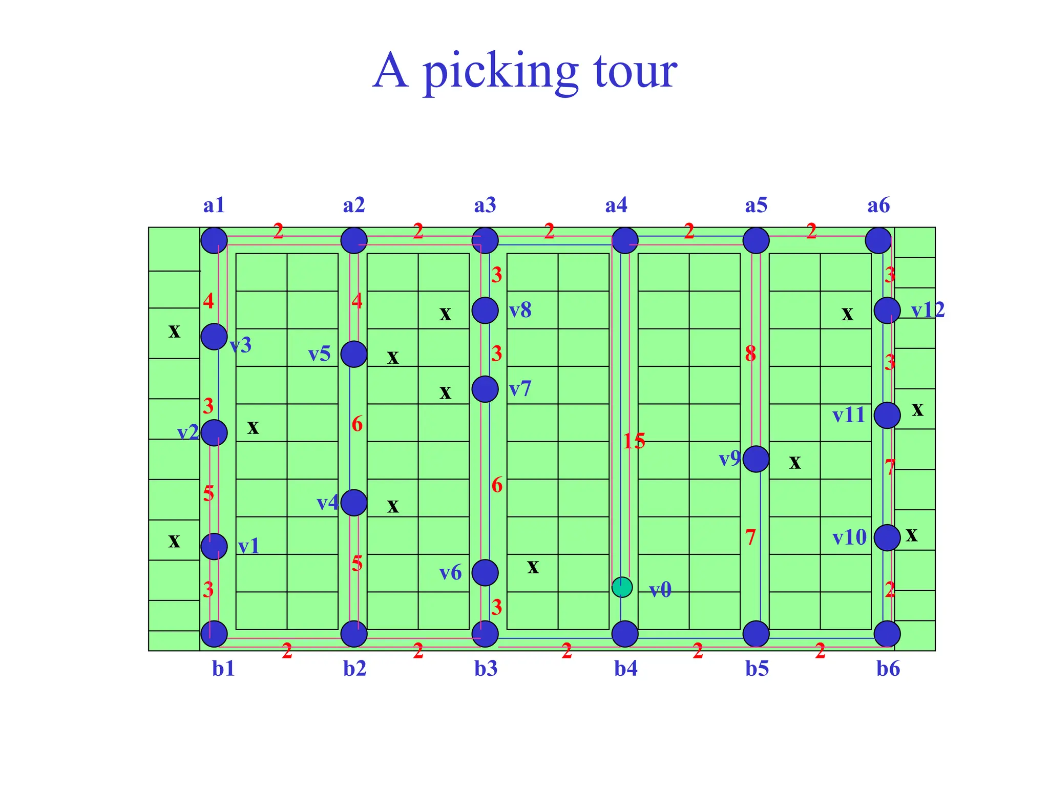
28. A picking tour
x
x
x
x
x
x
x
x
x
x
x
x
b1 b2 b3 b4 b5 b6
a1 a2 a3 a4 a5 a6
v0
v1
v2
v3
v4
v5
v6
v7
v8
v9
v10
v11
v12
2
2
2 2 2
2
7
3
3
2 2 2
2 2
3
5
3
4 4
6
5
3
6
3
3
15
8
7

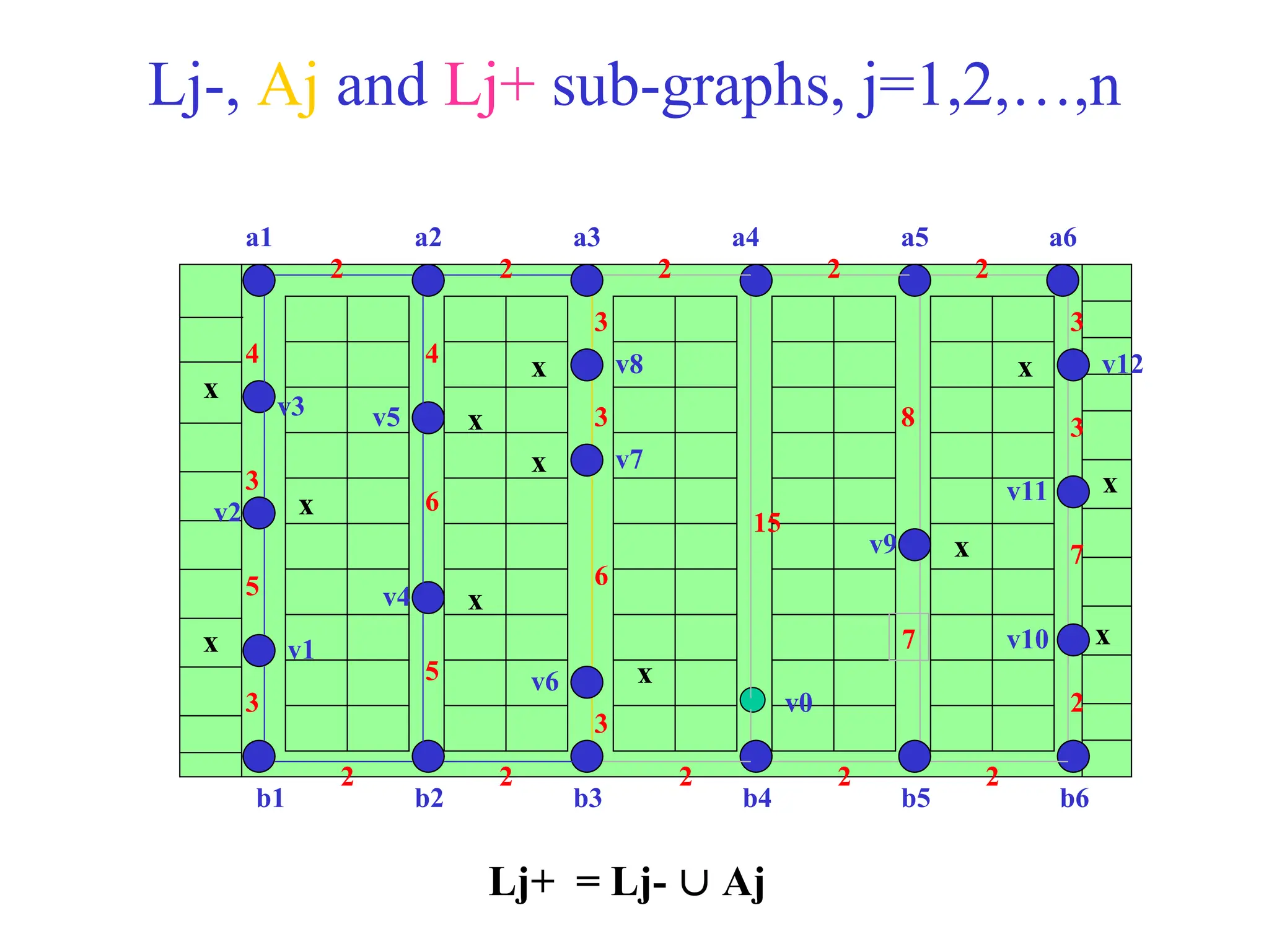
29. Lj-, Aj and Lj+ sub-graphs, j=1,2,…,n
x
x
x
x
x
x
x
x
x
x
x
x
b1 b2 b3 b4 b5 b6
a1 a2 a3 a4 a5 a6
v0
v1
v2
v3
v4
v5
v6
v7
v8
v9
v10
v11
v12
2
2
2 2 2
2
7
3
3
2 2 2
2 2
3
5
3
4 4
6
5
3
6
3
3
15
8
7
Lj+ = Lj-  Aj

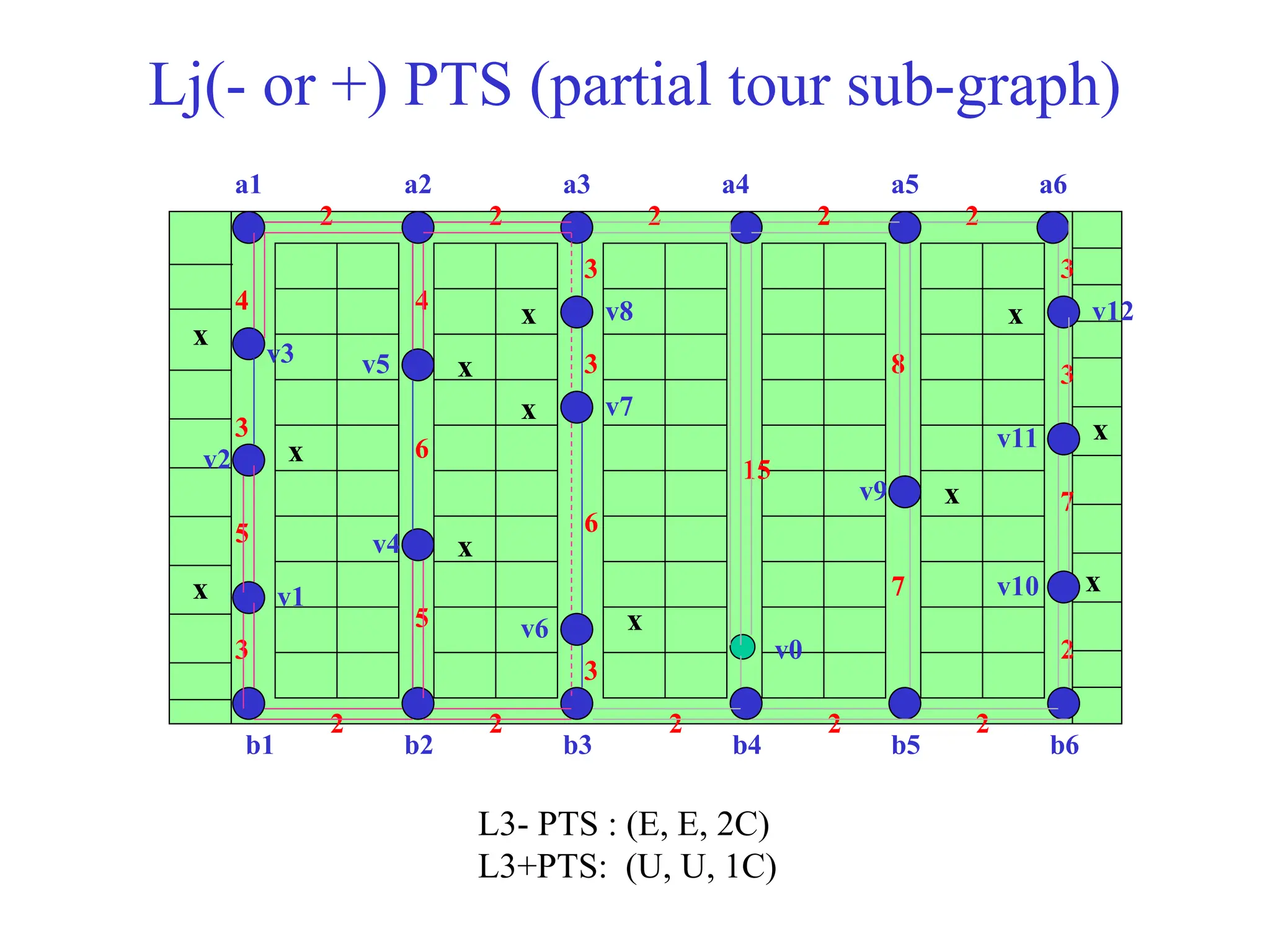
30. Lj(- or +) PTS (partial tour sub-graph)
x
x
x
x
x
x
x
x
x
x
x
x
b1 b2 b3 b4 b5 b6
a1 a2 a3 a4 a5 a6
v0
v1
v2
v3
v4
v5
v6
v7
v8
v9
v10
v11
v12
2
2
2 2 2
2
7
3
3
2 2 2
2 2
3
5
3
4 4
6
5
3
6
3
3
15
8
7
L3- PTS : (E, E, 2C)
L3+PTS: (U, U, 1C)

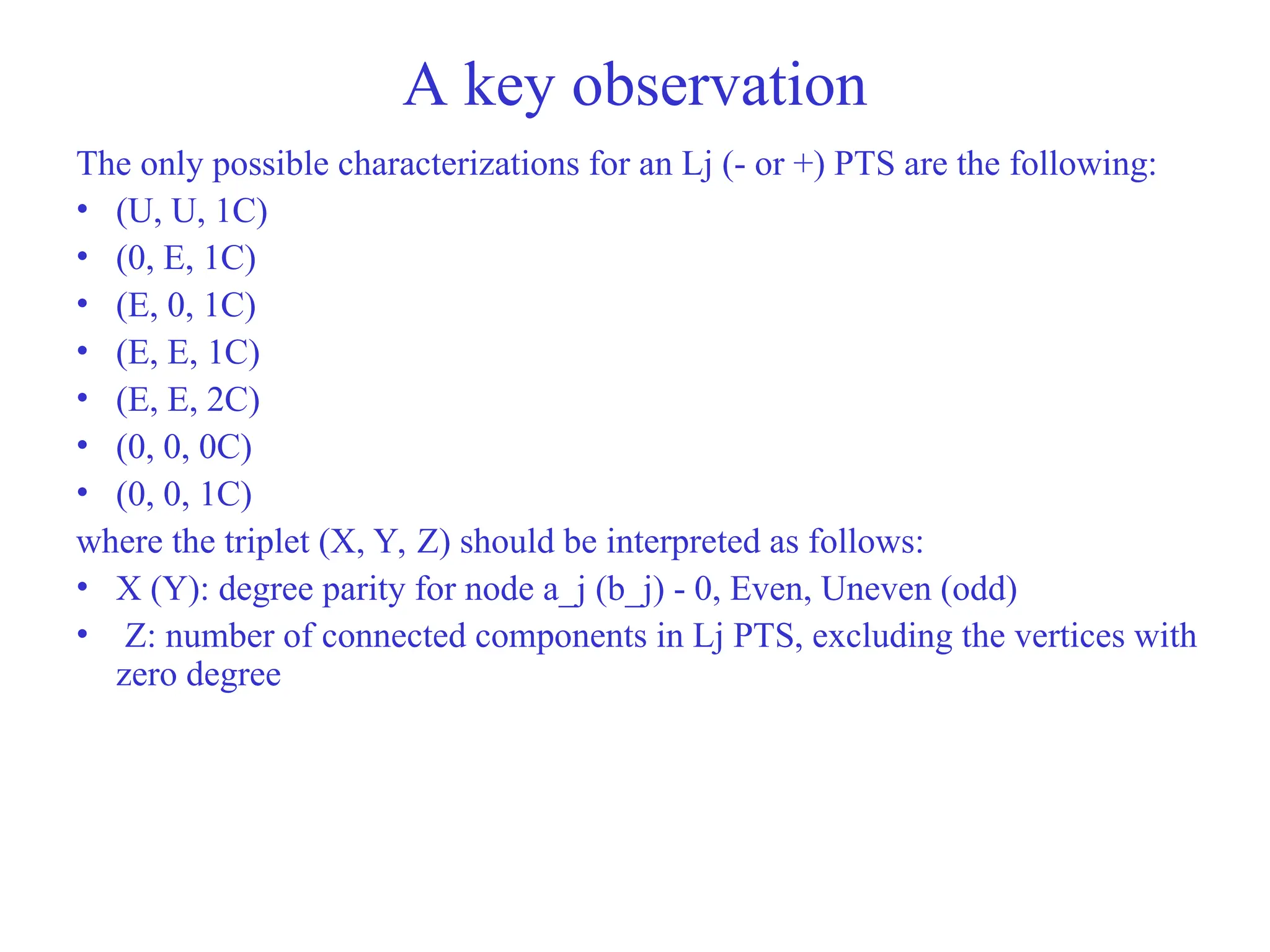
31. A key observation
The only possible characterizations for an Lj (- or +) PTS are the following:
• (U, U, 1C)
• (0, E, 1C)
• (E, 0, 1C)
• (E, E, 1C)
• (E, E, 2C)
• (0, 0, 0C)
• (0, 0, 1C)
where the triplet (X, Y, Z) should be interpreted as follows:
• X (Y): degree parity for node a_j (b_j) - 0, Even, Uneven (odd)
• Z: number of connected components in Lj PTS, excluding the vertices with
zero degree

32. Going from Lj- to Lj+…
a_j a_j a_j
a_j a_j a_j
b_j b_j b_j b_j b_j b_j
(I-i) (I-ii) (I-iii) (I-iv) (I-v) (I-vi)

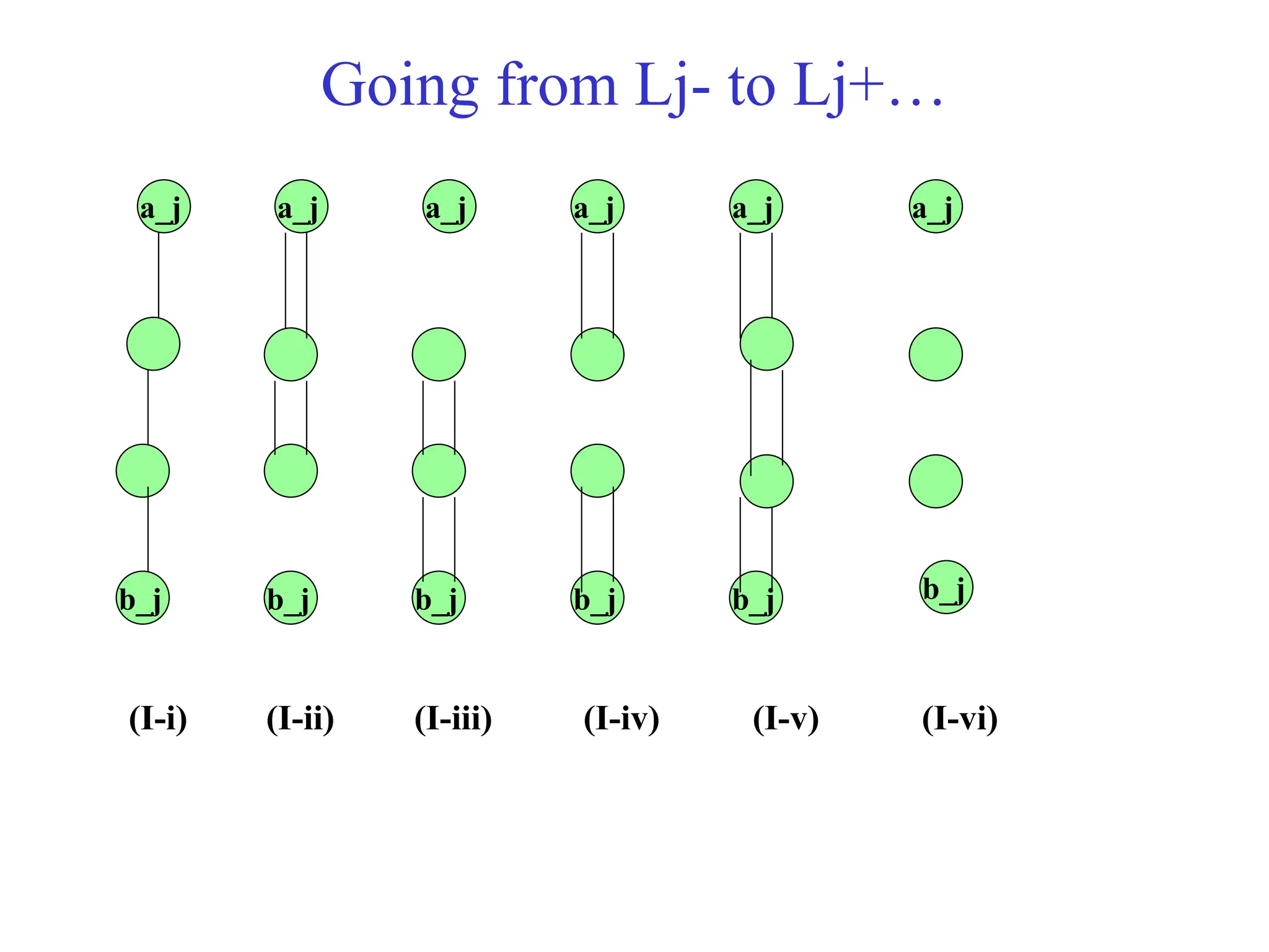
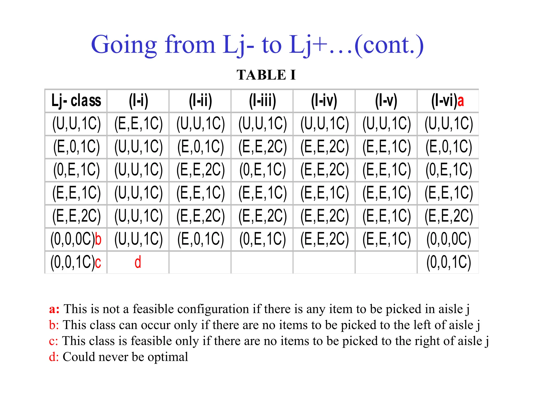
33. Going from Lj- to Lj+…(cont.)
Lj- class (I-i) (I-ii) (I-iii) (I-iv) (I-v) (I-vi)a
(U,U,1C) (E,E,1C) (U,U,1C) (U,U,1C) (U,U,1C) (U,U,1C) (U,U,1C)
(E,0,1C) (U,U,1C) (E,0,1C) (E,E,2C) (E,E,2C) (E,E,1C) (E,0,1C)
(0,E,1C) (U,U,1C) (E,E,2C) (0,E,1C) (E,E,2C) (E,E,1C) (0,E,1C)
(E,E,1C) (U,U,1C) (E,E,1C) (E,E,1C) (E,E,1C) (E,E,1C) (E,E,1C)
(E,E,2C) (U,U,1C) (E,E,2C) (E,E,2C) (E,E,2C) (E,E,1C) (E,E,2C)
(0,0,0C)b (U,U,1C) (E,0,1C) (0,E,1C) (E,E,2C) (E,E,1C) (0,0,0C)
(0,0,1C)c d (0,0,1C)
a: This is not a feasible configuration if there is any item to be picked in aisle j
b: This class can occur only if there are no items to be picked to the left of aisle j
c: This class is feasible only if there are no items to be picked to the right of aisle j
d: Could never be optimal
TABLE I

34. Going from Lj+ to L(j+1)-…
a_j+1
a_j
b_j b_j+1
a_j+1
a_j
b_j b_j+1
a_j+1
a_j
b_j b_j+1
a_j+1
a_j
b_j b_j+1
a_j+1
a_j
b_j b_j+1
(II-i) (II-ii) (II-iii)
(II-iv) (II-v)

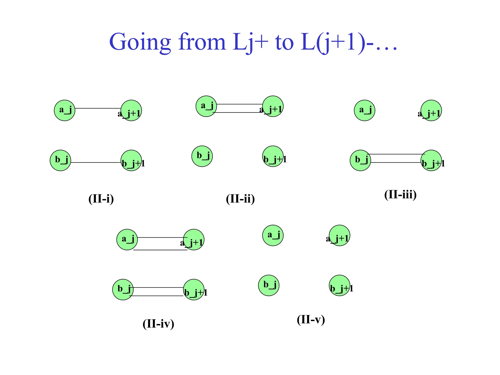
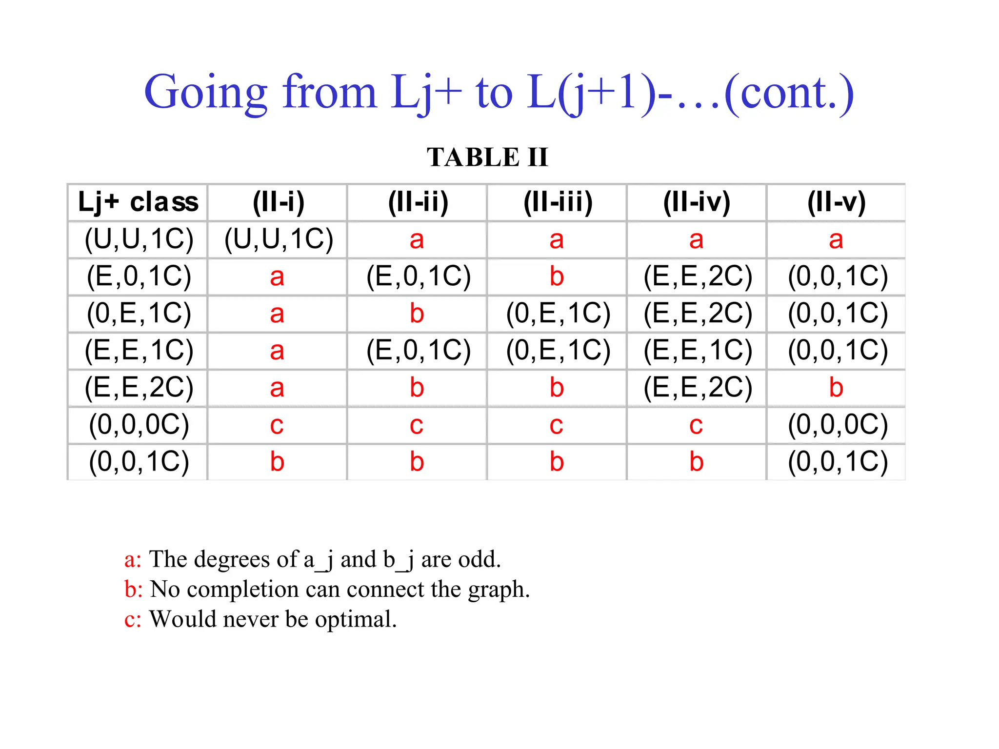
35. Going from Lj+ to L(j+1)-…(cont.)
Lj+ class (II-i) (II-ii) (II-iii) (II-iv) (II-v)
(U,U,1C) (U,U,1C) a a a a
(E,0,1C) a (E,0,1C) b (E,E,2C) (0,0,1C)
(0,E,1C) a b (0,E,1C) (E,E,2C) (0,0,1C)
(E,E,1C) a (E,0,1C) (0,E,1C) (E,E,1C) (0,0,1C)
(E,E,2C) a b b (E,E,2C) b
(0,0,0C) c c c c (0,0,0C)
(0,0,1C) b b b b (0,0,1C)
a: The degrees of a_j and b_j are odd.
b: No completion can connect the graph.
c: Would never be optimal.
TABLE II

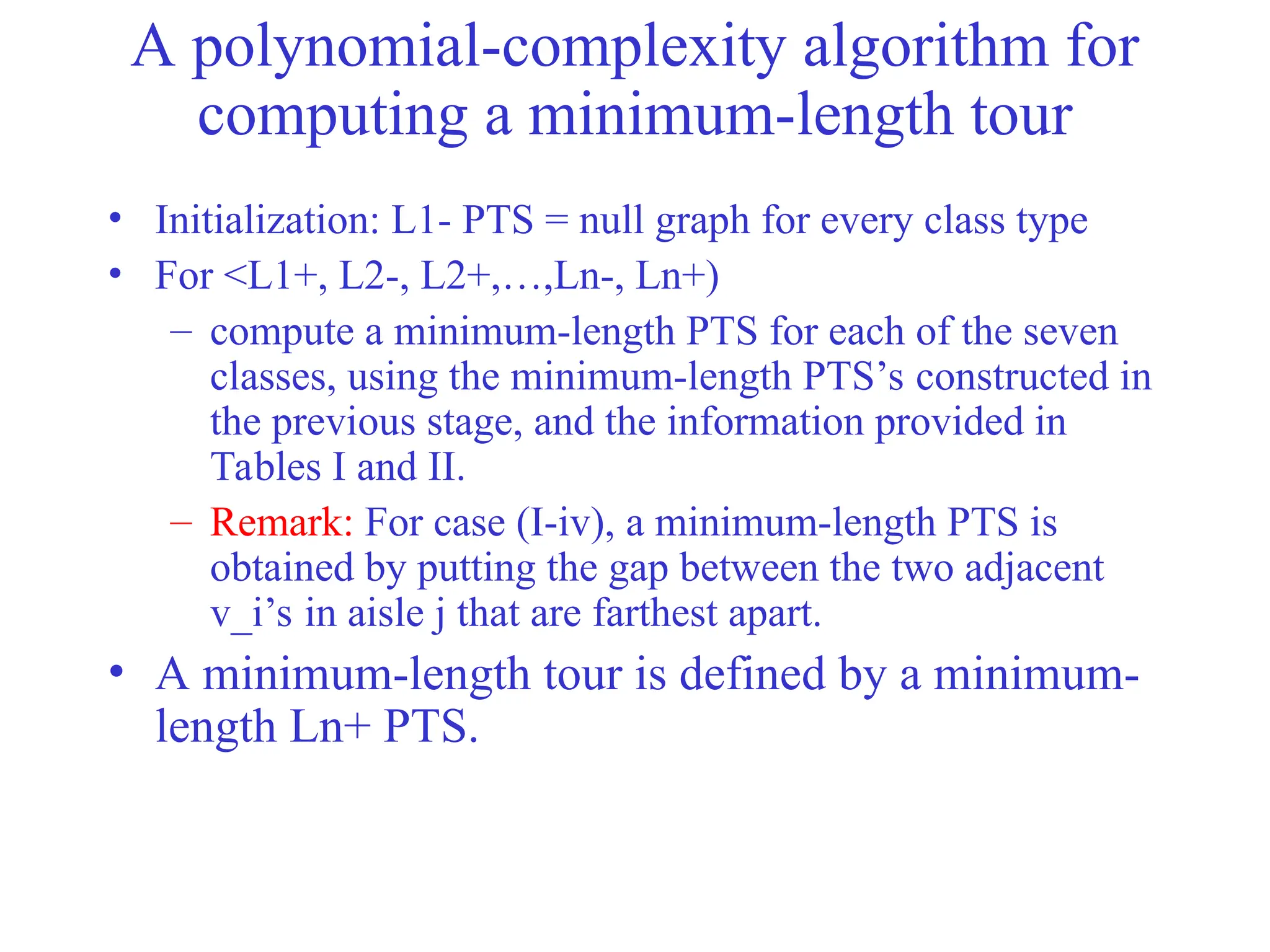
36. A polynomial-complexity algorithm for
computing a minimum-length tour
• Initialization: L1- PTS = null graph for every class type
• For <L1+, L2-, L2+,…,Ln-, Ln+)
– compute a minimum-length PTS for each of the seven
classes, using the minimum-length PTS’s constructed in
the previous stage, and the information provided in
Tables I and II.
– Remark: For case (I-iv), a minimum-length PTS is
obtained by putting the gap between the two adjacent
v_i’s in aisle j that are farthest apart.
• A minimum-length tour is defined by a minimum-
length Ln+ PTS.

37. Example (c.f., slide 8)
PTS-class L1- L1+ L2- L2+ L3- L3+
1.(U,U,1C) 15,-,I-I 19,1,II-I 37,1,I-iv 41,1,II-I 53,2,I-I
2.(E,0,1C) 24,-,I-ii 28,2,II-ii 48,2,I-ii 38,4,II-ii 62,2,I-ii
3.(0,E,1C) 22,-,I-iii 26,3,II-iii 48,3,I-iii 38,4,II-iii 62,3,I-iii
4.(E,E,1C) 30,-,I-v 38,4,II-iv 34,1,I-I 42,4,II-iv 56,1,I-I
5.(E,E,2C) 20,-,I-iv 28,5,II-iv 44,3,I-? 52,5,II-iv 56,2,I-iv
6.(0,0,0C)
7.(0,0,1C) 22,3,II-v 34,4,II-v
PTS-class L4- L4+ L5- L5+ L6- L6+
1.(U,U,1C) 57,1,II-I 57,1,I-iii 61,1,II-I 75,1,I-iii 79,1,II-I 95,1,I-iv
2.(E,0,1C) 60,4,II-ii 90,2,I-ii 68,4,II-ii 84,2,I-ii 80,4,II-ii 106,2,I-ii
3.(0,E,1C) 60,4,II-iii 60,3,I-iii 64,3,II-iii 78,2,I-iii 80,4,II-iii 104,3,I-iii
4.(E,E,1C) 64,4,II-iv 64,4,I-iii 72,4,II-iv 76,1,I-I 84,4,II-iv 94,1,I,I
5.(E,E,2C) 64,5,II-iv 60,2,I-iii 68,3,II-iv 80,3,I-ii 86,3,II-iv 96,2,I,iv
6.(0,0,0C)
7.(0,0,1C) 56,4,II-v 60,3,II-v 76,4,II-v

38. Example: The optimal tour
x
x
x
x
x
x
x
x
x
x
x
x
b1 b2 b3 b4 b5 b6
a1 a2 a3 a4 a5 a6
v0
v1
v2
v3
v4
v5
v6
v7
v8
v9
v10
v11
v12
2
2
2 2 2
2
7
3
3
2 2 2
2 2
3
5
3
4 4
6
5
3
6
3
3
15
8
7
0