Material Requirement Process

1. Material Requirements
Material Requirements
Planning
Planning
Dr. Everette S. Gardner, Jr.

2. MRP 2
End
item
Component
Raw
material
R
Time
LT
LT
R
Time
LT
R
Time
LT
Order point system with dependent demand

3. MRP 3
End
item
Component
Raw
material
R
Time
Time
Time
The MRP approach

4. MRP 4
The simultaneous probability
problem
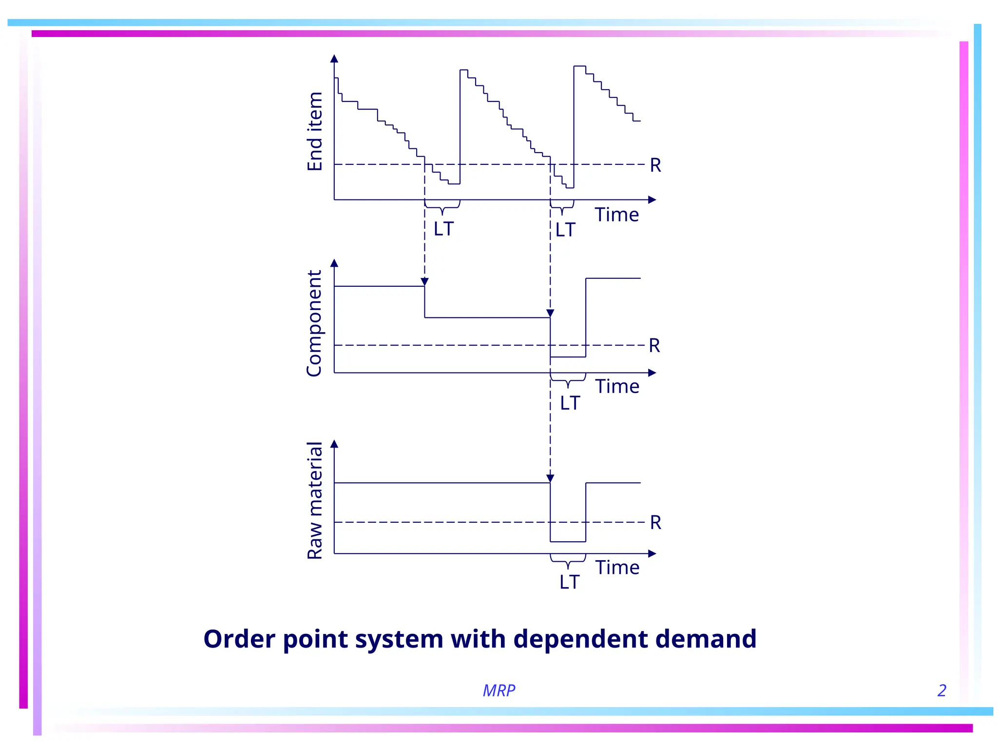
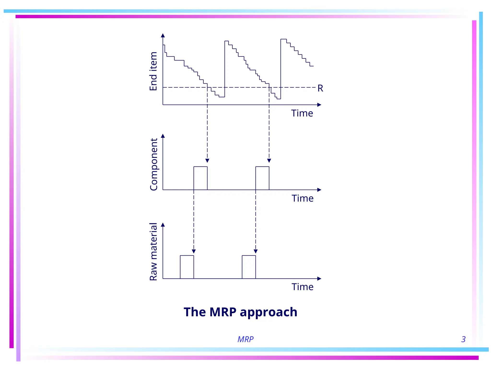
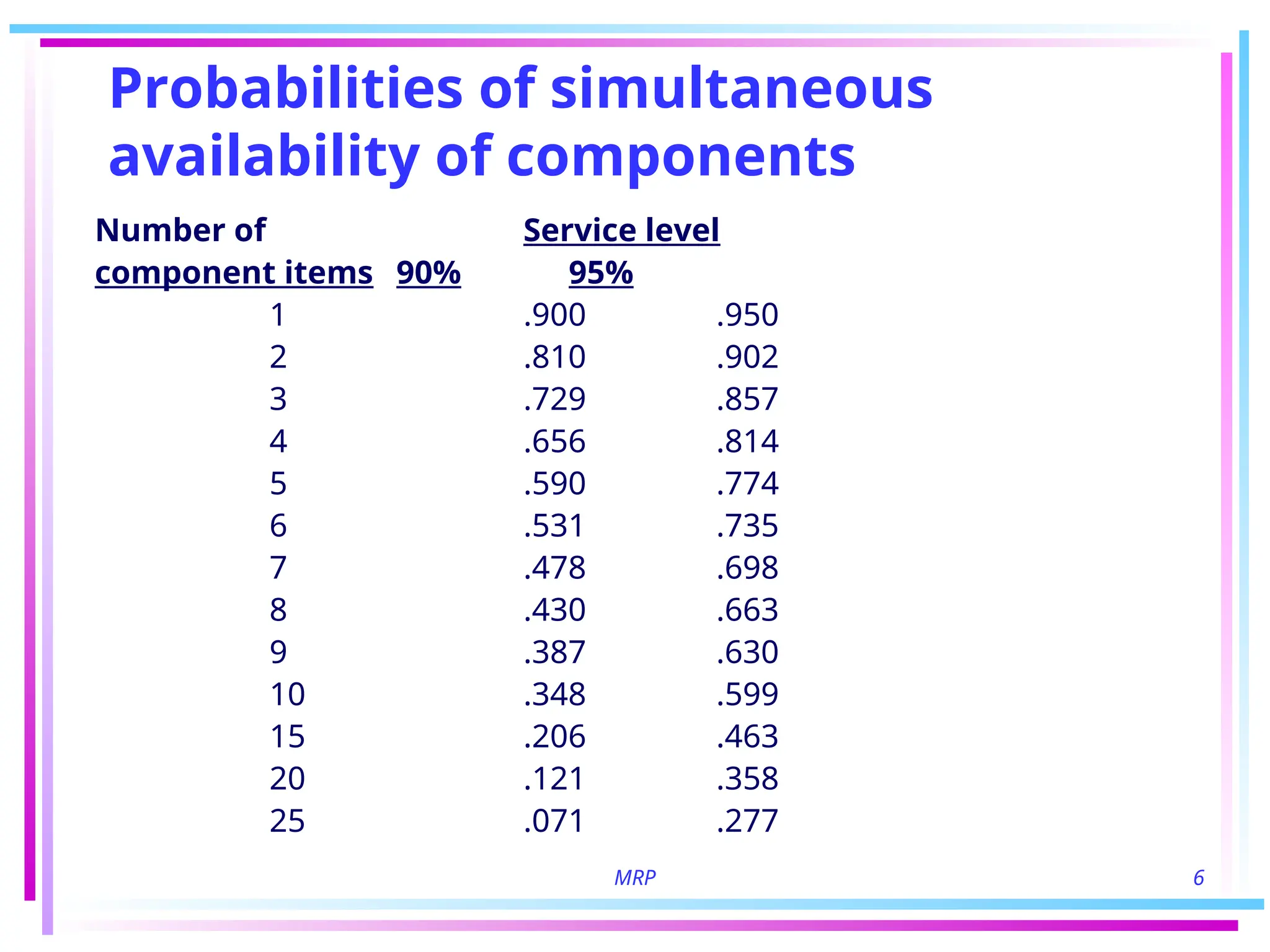
• When components are ordered independently with an order point
system, the probability that all will be in stock at the same time is
much lower than the probabilities for individual components
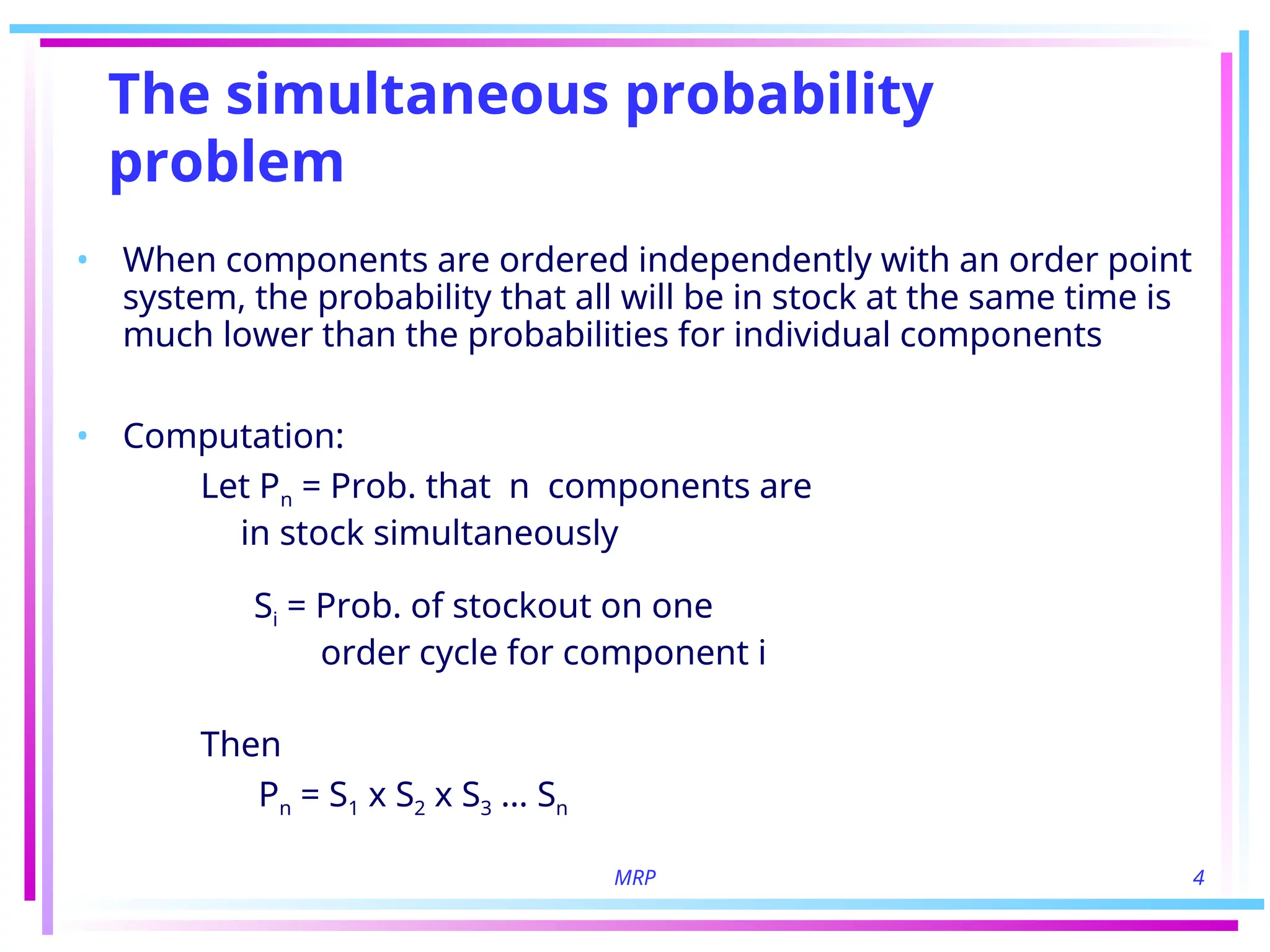
• Computation:
Let Pn = Prob. that n components are
in stock simultaneously
Si = Prob. of stockout on one
order cycle for component i
Then
Pn = S1 x S2 x S3 … Sn

5. MRP 5
The simultaneous probability
problem (cont.)
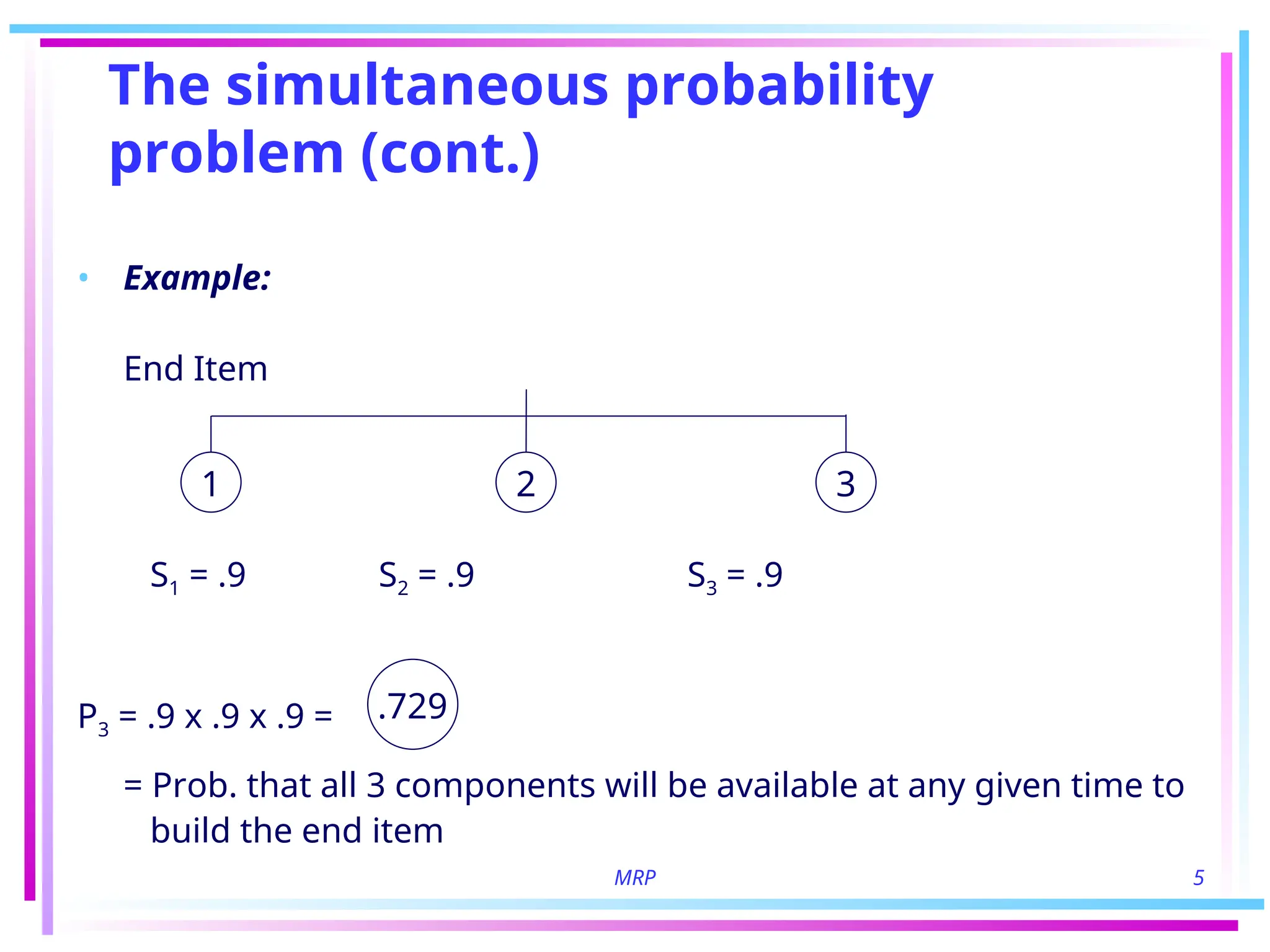
• Example:
End Item
S1 = .9 S2 = .9 S3 = .9
P3 = .9 x .9 x .9 =
= Prob. that all 3 components will be available at any given time to
build the end item
1 2 3
.729

6. MRP 6
Probabilities of simultaneous
availability of components
Number of Service level
component items 90% 95%
1 .900 .950
2 .810 .902
3 .729 .857
4 .656 .814
5 .590 .774
6 .531 .735
7 .478 .698
8 .430 .663
9 .387 .630
10 .348 .599
15 .206 .463
20 .121 .358
25 .071 .277

7. MRP 7
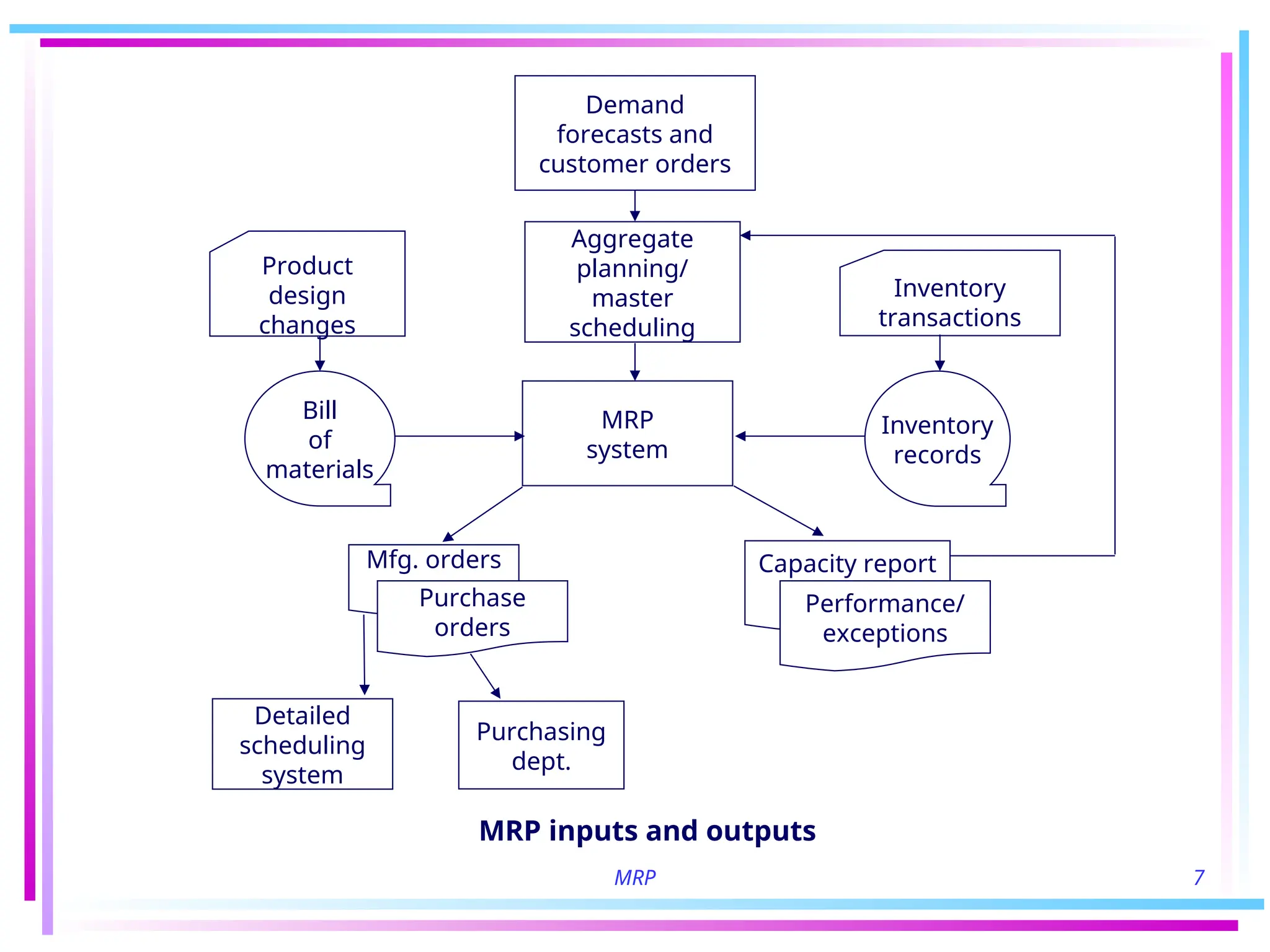
Mfg. orders
Demand
forecasts and
customer orders
Aggregate
planning/
master
scheduling
Product
design
changes
Inventory
transactions
Bill
of
materials
MRP
system
Inventory
records
Purchase
orders
Capacity report
Performance/
exceptions
Detailed
scheduling
system
Purchasing
dept.
MRP inputs and outputs

8. MRP 8
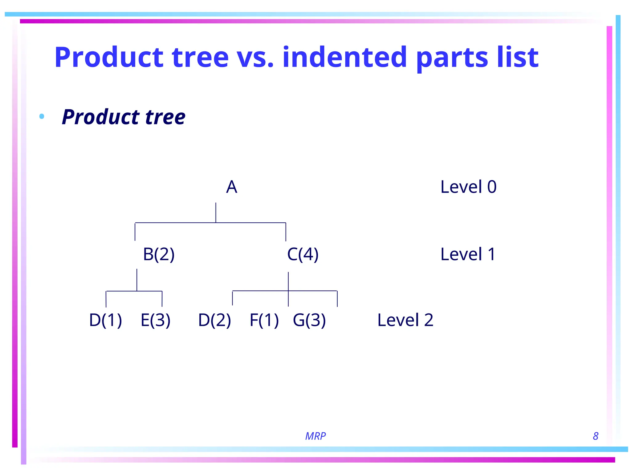
Product tree vs. indented parts list
• Product tree
A Level 0
B(2) C(4) Level 1
D(1) E(3) D(2) F(1) G(3) Level 2

9. MRP 9
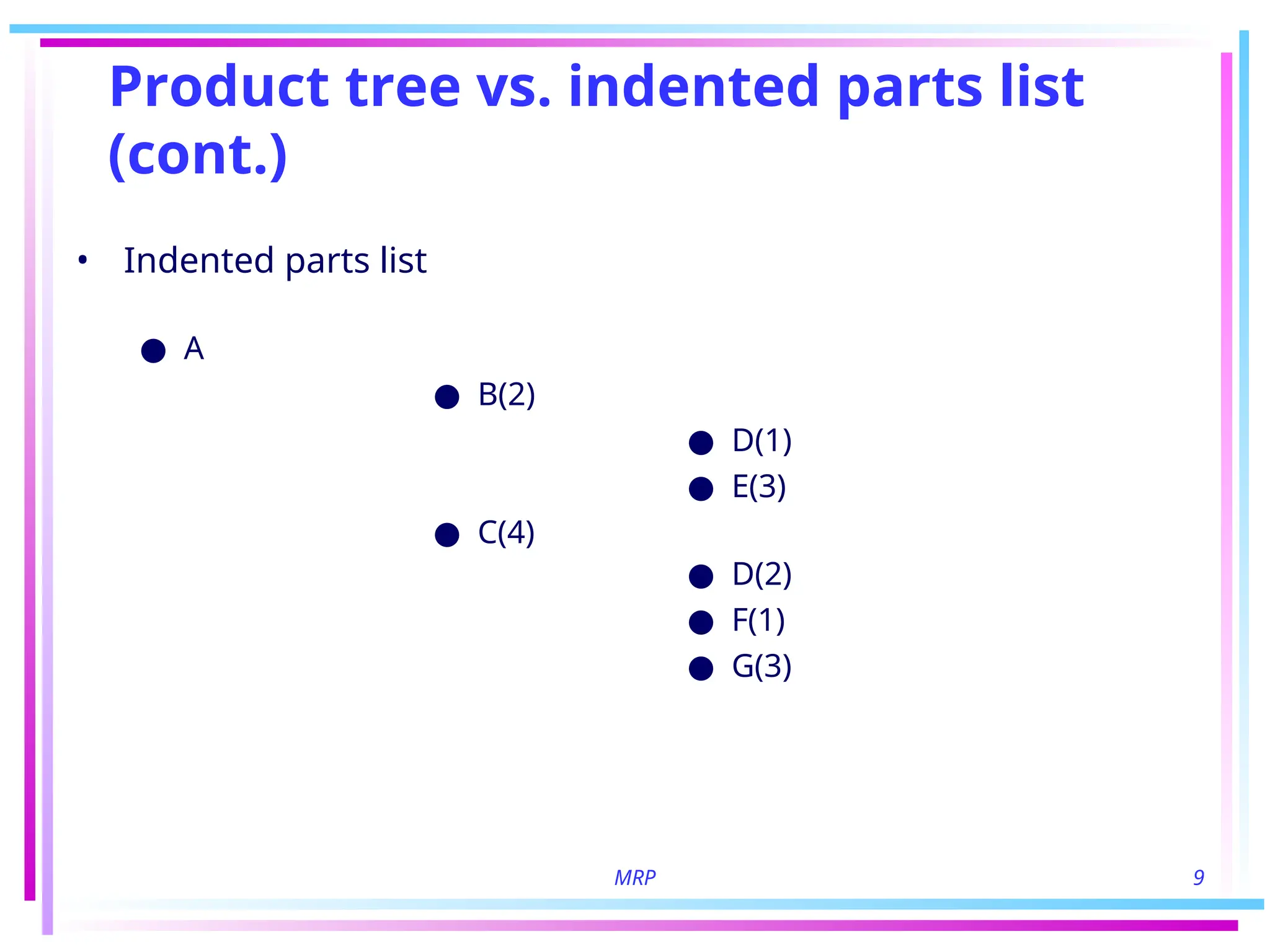
Product tree vs. indented parts list
(cont.)
• Indented parts list
● A
● B(2)
● D(1)
● E(3)
● C(4)
● D(2)
● F(1)
● G(3)

10. MRP 10
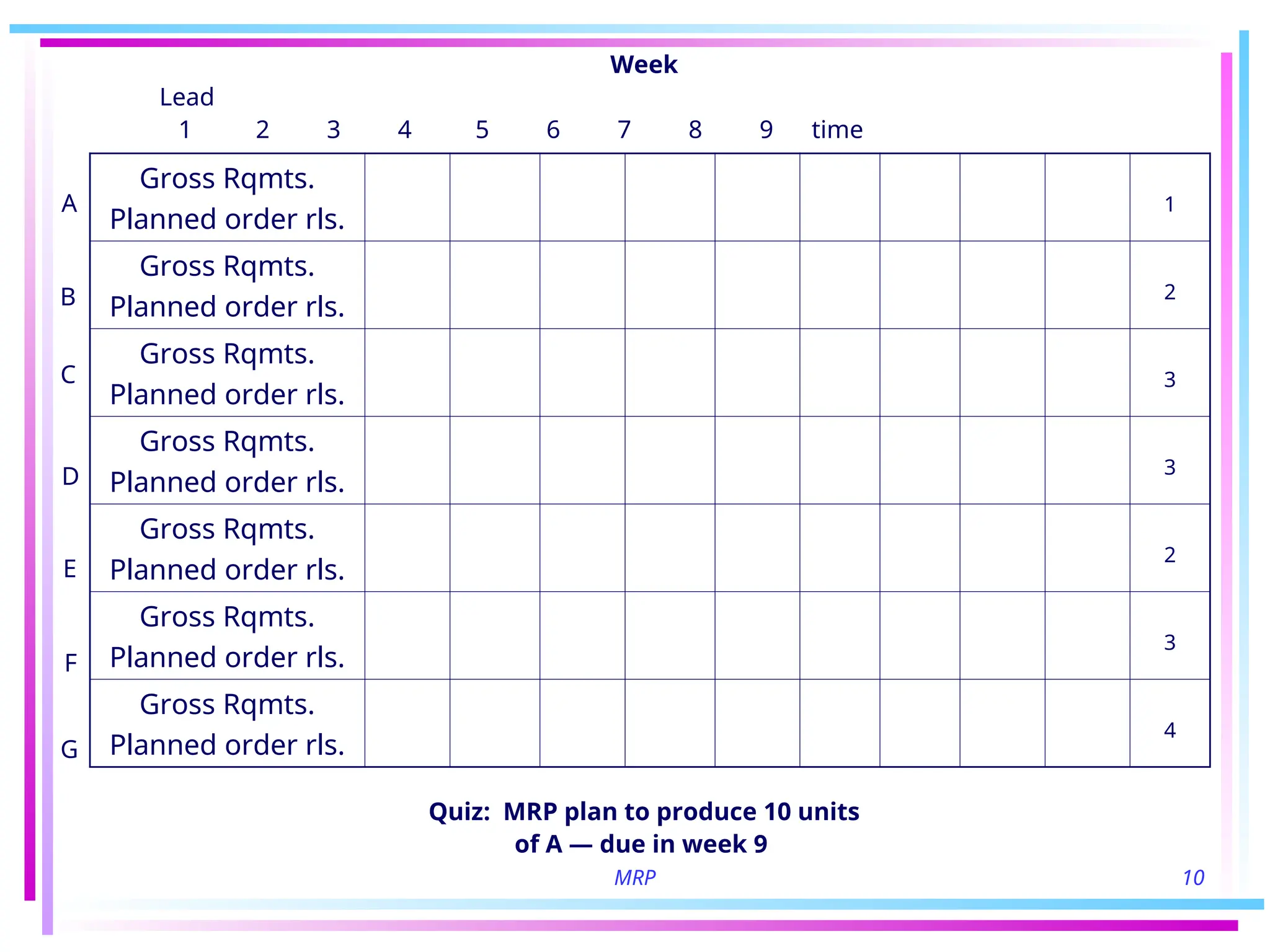
Week
Lead
1 2 3 4 5 6 7 8 9 time
Quiz: MRP plan to produce 10 units
of A — due in week 9
Gross Rqmts.
Planned order rls.
1
Gross Rqmts.
Planned order rls.
2
Gross Rqmts.
Planned order rls.
3
Gross Rqmts.
Planned order rls.
3
Gross Rqmts.
Planned order rls.
2
Gross Rqmts.
Planned order rls.
3
Gross Rqmts.
Planned order rls.
4
A
B
C
G
F
E
D

11. MRP 11
Problems in requirements
computations
• Product structure
• Recurring requirements within the planning horizon
• Multilevel items
• Rescheduling open orders

12. MRP 12
Product structure
• Bills of material are hierarchical with distinct levels
• To compute requirements, always proceed down bill of
materials, processing all requirements at one level before
starting another

13. MRP 13
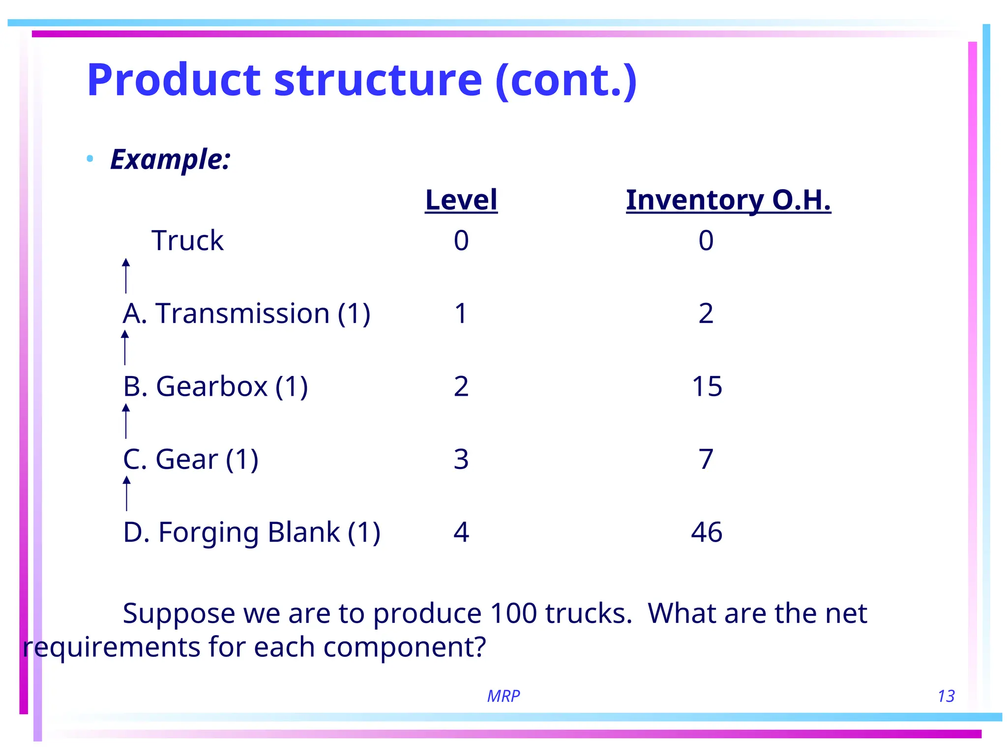
Product structure (cont.)
• Example:
Level Inventory O.H.
Truck 0 0
A. Transmission (1) 1 2
B. Gearbox (1) 2 15
C. Gear (1) 3 7
D. Forging Blank (1) 4 46
Suppose we are to produce 100 trucks. What are the net
requirements for each component?

14. MRP 14
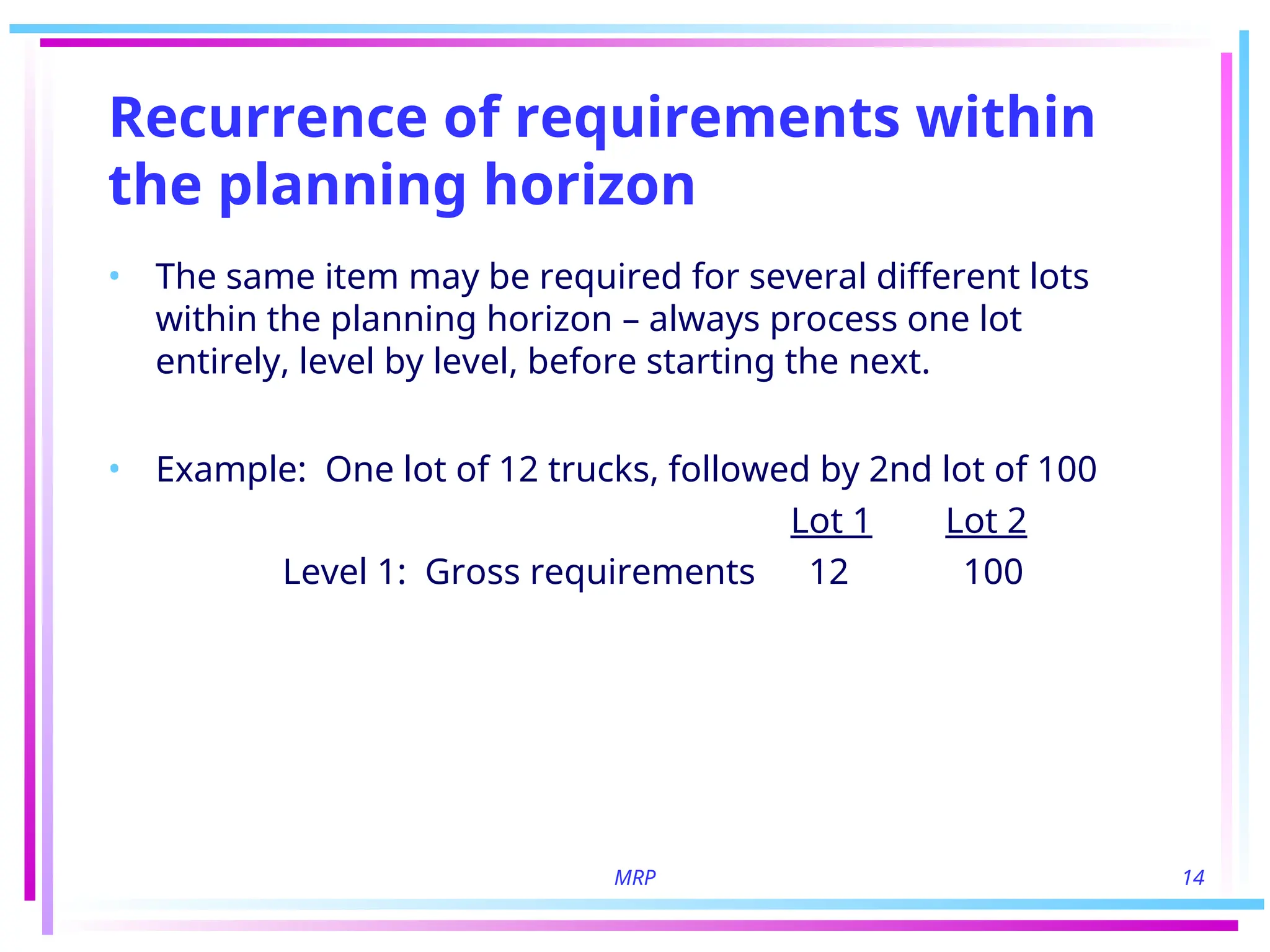
Recurrence of requirements within
the planning horizon
• The same item may be required for several different lots
within the planning horizon – always process one lot
entirely, level by level, before starting the next.
• Example: One lot of 12 trucks, followed by 2nd lot of 100
Lot 1 Lot 2
Level 1: Gross requirements 12 100

15. MRP 15
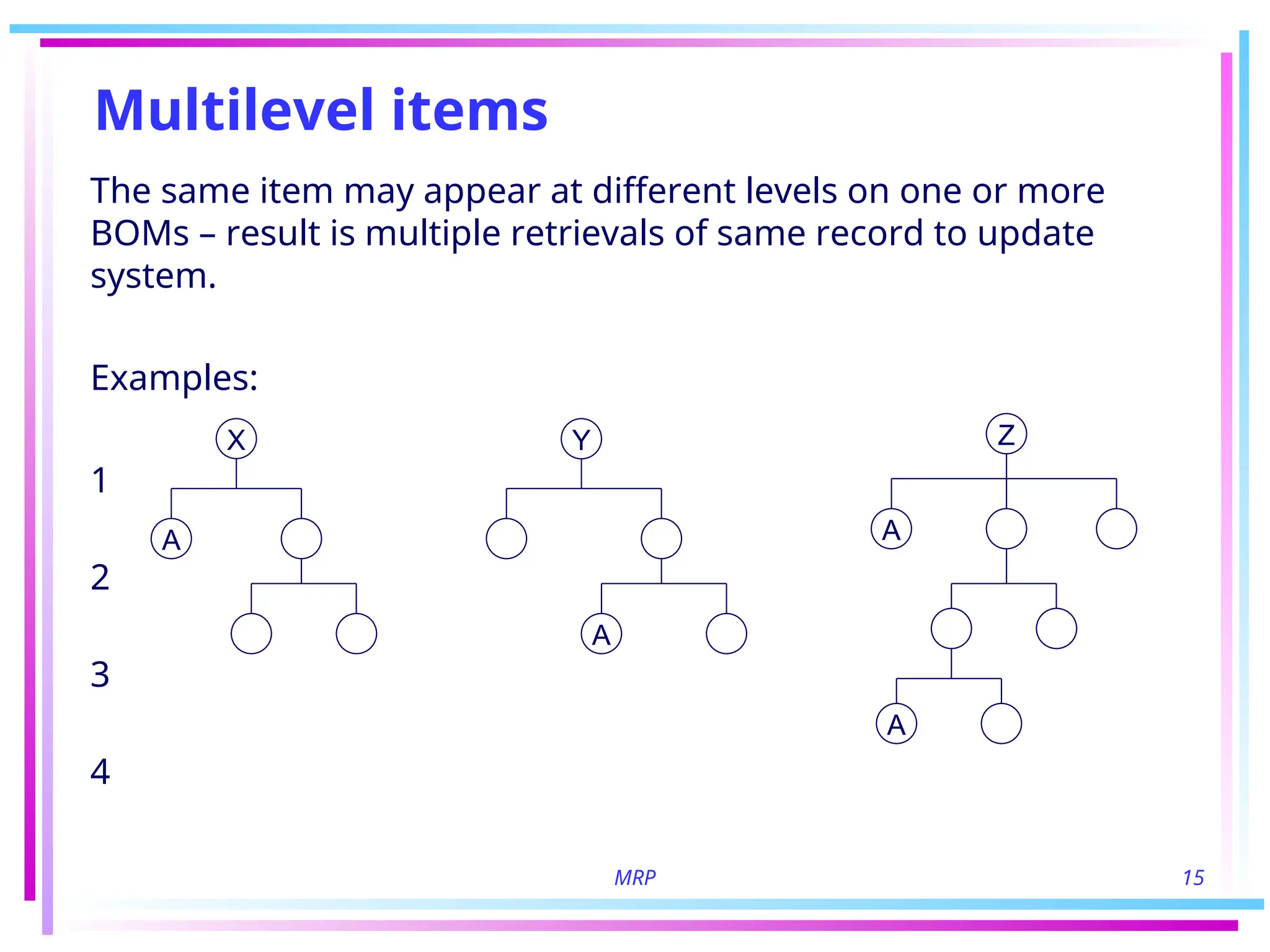
Multilevel items
The same item may appear at different levels on one or more
BOMs – result is multiple retrievals of same record to update
system.
Examples:
1
2
3
4
X
A
Y
A
Z
A
A

16. MRP 16
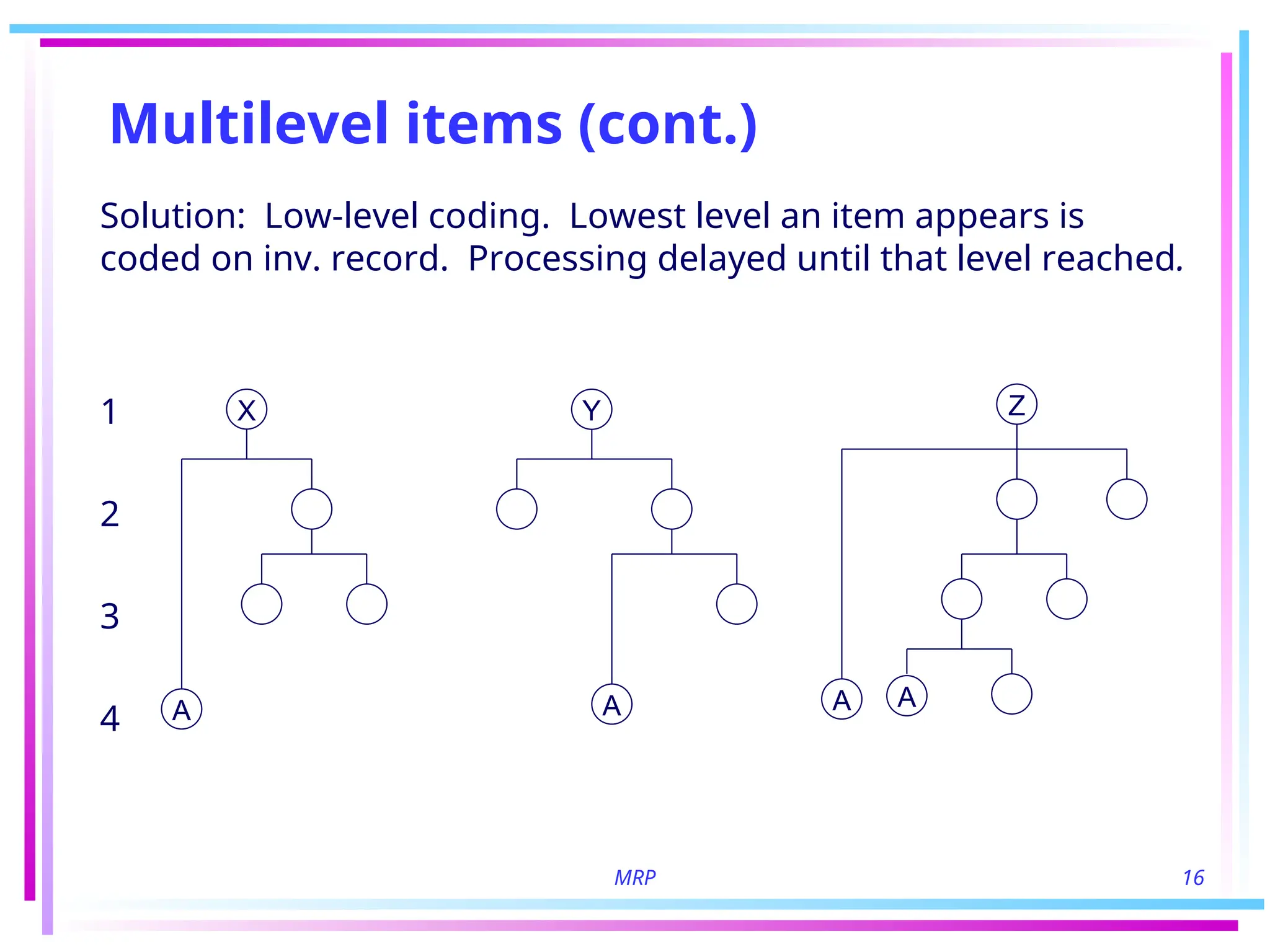
Multilevel items (cont.)
Solution: Low-level coding. Lowest level an item appears is
coded on inv. record. Processing delayed until that level reached.
1
2
3
4
X
A
Y
A
Z
A A

17. MRP 17
Rescheduling open orders
• Tests for open order misalignment:
1. Are open orders scheduled for periods following the period
in which a net requirement appears?
2. Is an open order scheduled for a period in which gross
requirement inv. O. H. at end of preceding period?
≤
3. Is lead-time sufficient?

18. MRP 18
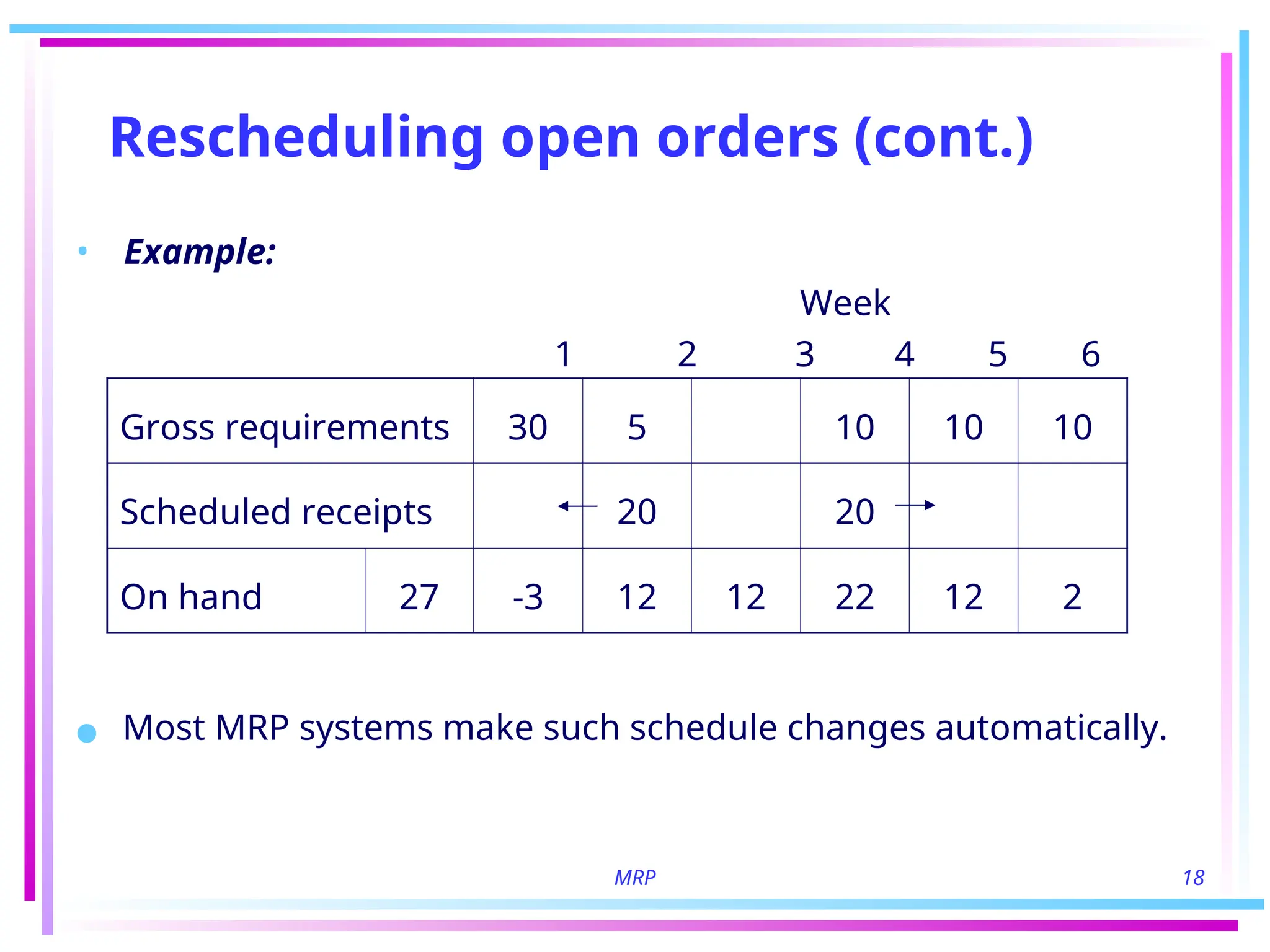
Rescheduling open orders (cont.)
• Example:
Week
1 2 3 4 5 6
● Most MRP systems make such schedule changes automatically.
Gross requirements 30 5 10 10 10
Scheduled receipts 20 20
On hand 27 -3 12 12 22 12 2

19. MRP 19
Tactical questions in MRP
• Regeneration vs. net change
• Lot sizing
• Safety stocks

20. MRP 20
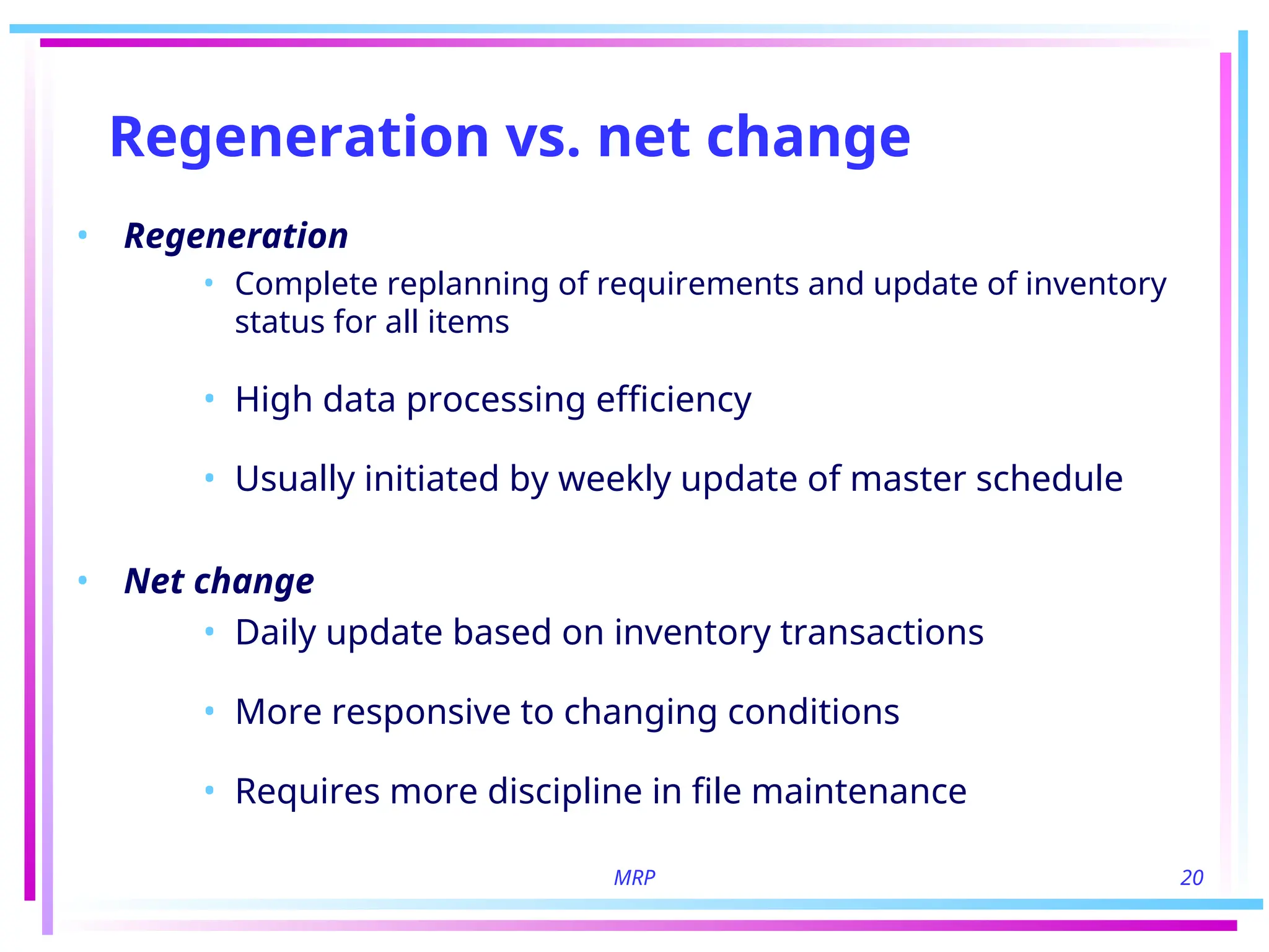
Regeneration vs. net change
• Regeneration
• Complete replanning of requirements and update of inventory
status for all items
• High data processing efficiency
• Usually initiated by weekly update of master schedule
• Net change
• Daily update based on inventory transactions
• More responsive to changing conditions
• Requires more discipline in file maintenance

21. MRP 21
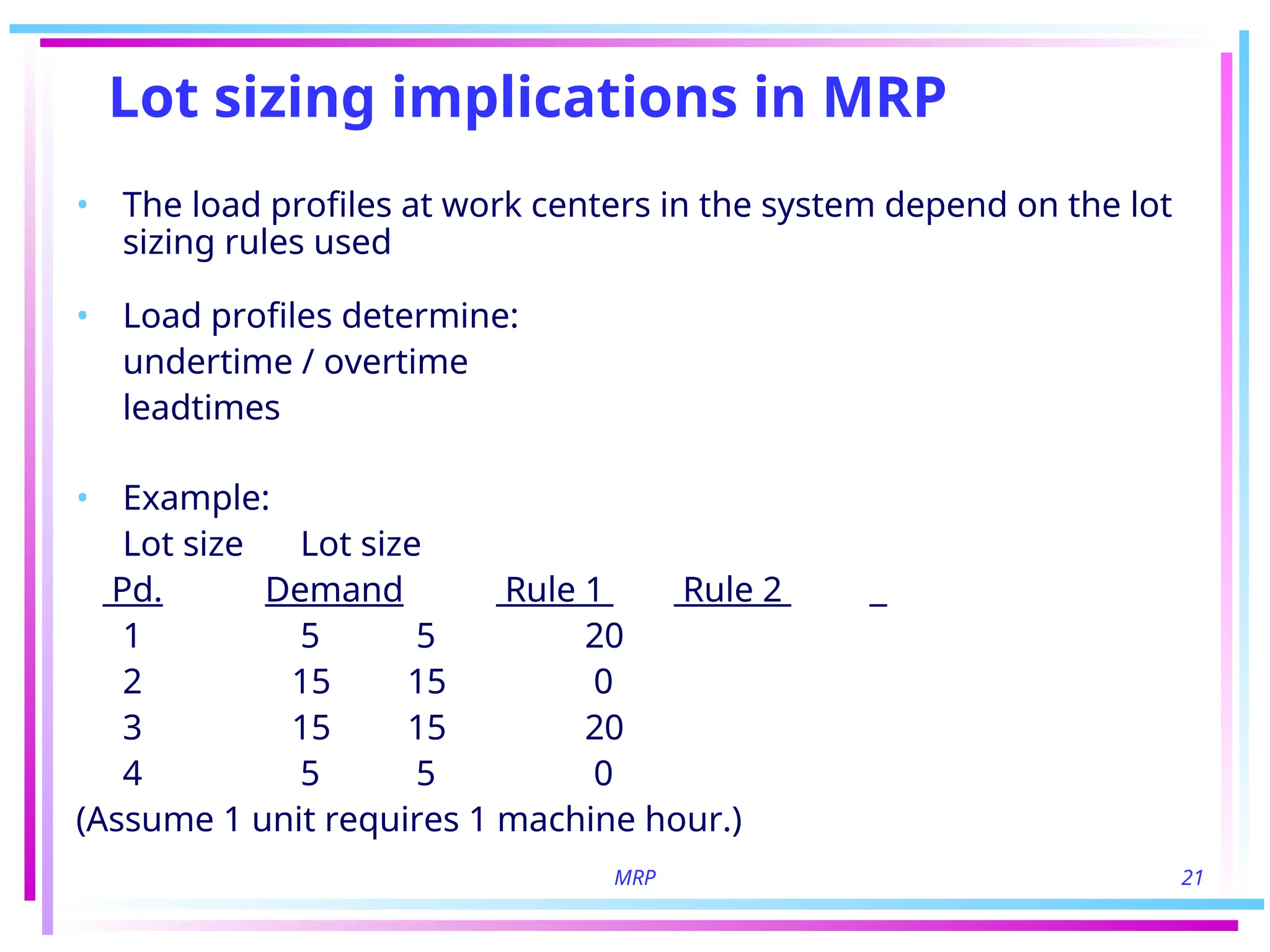
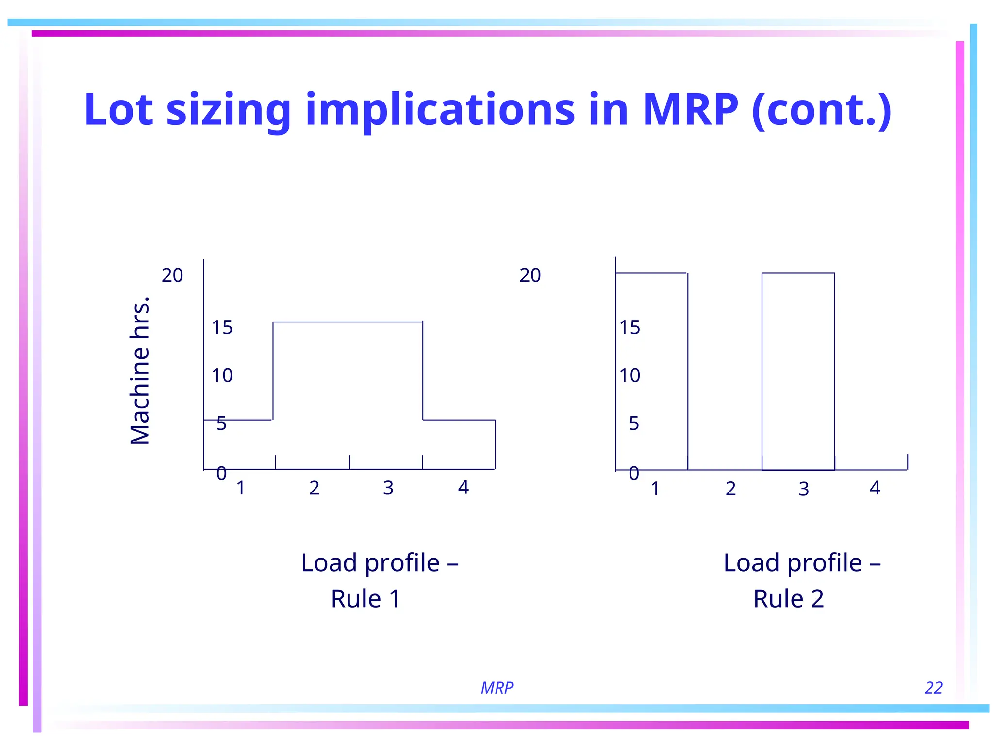
Lot sizing implications in MRP
• The load profiles at work centers in the system depend on the lot
sizing rules used
• Load profiles determine:
undertime / overtime
leadtimes
• Example:
Lot size Lot size
Pd. Demand Rule 1 Rule 2
1 5 5 20
2 15 15 0
3 15 15 20
4 5 5 0
(Assume 1 unit requires 1 machine hour.)

22. MRP 22
Lot sizing implications in MRP (cont.)
20 20
15 15
10 10
5 5
0 0
Load profile – Load profile –
Rule 1 Rule 2
Machine
hrs.
1 2 3 4 1 2 3 4

23. MRP 23
Lot sizing techniques used in MRP
systems
• Lot-for-lot (L4L) – most used
• Economic order quantity (EOQ)
• Period order quantity (POQ)

24. MRP 24
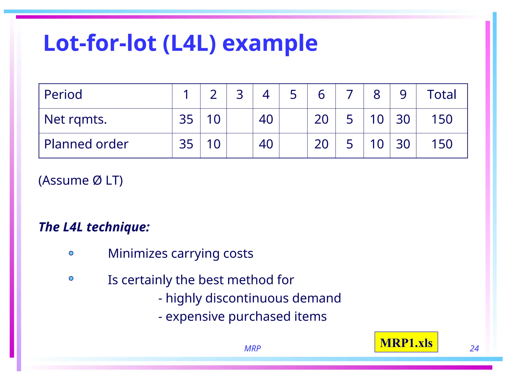
Lot-for-lot (L4L) example
(Assume Ø LT)
The L4L technique:
Minimizes carrying costs
Is certainly the best method for
- highly discontinuous demand
- expensive purchased items
Period 1 2 3 4 5 6 7 8 9 Total
Net rqmts. 35 10 40 20 5 10 30 150
Planned order 35 10 40 20 5 10 30 150
MRP1.xls

25. MRP 25
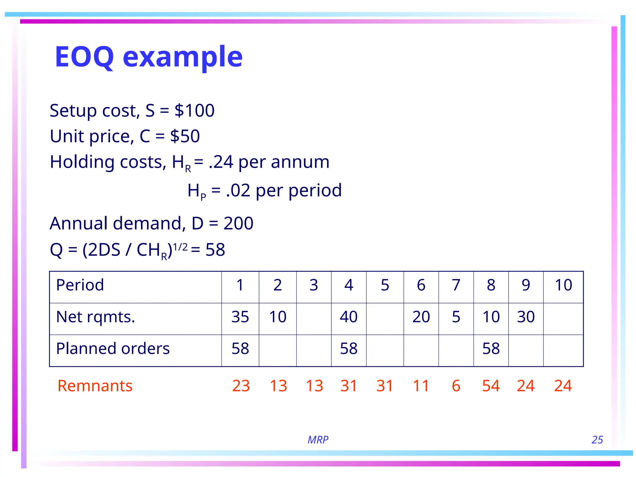
EOQ example
Setup cost, S = $100
Unit price, C = $50
Holding costs, HR = .24 per annum
HP = .02 per period
Annual demand, D = 200
Q = (2DS / CHR)1/2
= 58
Period 1 2 3 4 5 6 7 8 9 10
Net rqmts. 35 10 40 20 5 10 30
Planned orders 58 58 58
Remnants 23 13 13 31 31 11 6 54 24 24

26. MRP 26
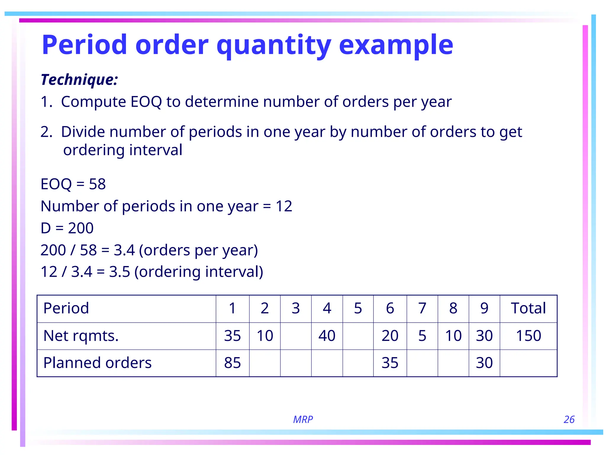
Period order quantity example
Technique:
1. Compute EOQ to determine number of orders per year
2. Divide number of periods in one year by number of orders to get
ordering interval
EOQ = 58
Number of periods in one year = 12
D = 200
200 / 58 = 3.4 (orders per year)
12 / 3.4 = 3.5 (ordering interval)
Period 1 2 3 4 5 6 7 8 9 Total
Net rqmts. 35 10 40 20 5 10 30 150
Planned orders 85 35 30

27. MRP 27
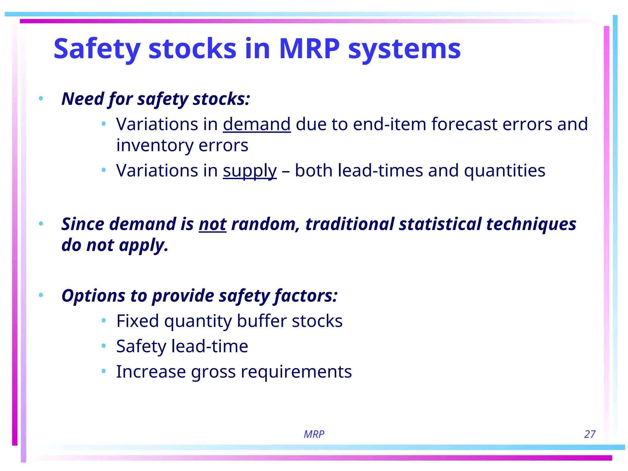
Safety stocks in MRP systems
• Need for safety stocks:
• Variations in demand due to end-item forecast errors and
inventory errors
• Variations in supply – both lead-times and quantities
• Since demand is not random, traditional statistical techniques
do not apply.
• Options to provide safety factors:
• Fixed quantity buffer stocks
• Safety lead-time
• Increase gross requirements

28. MRP 28
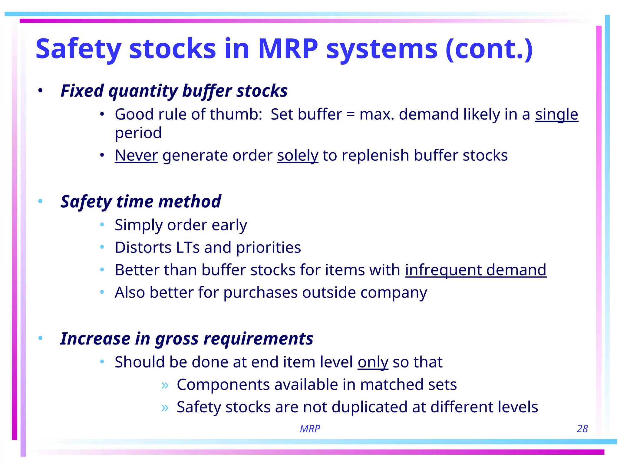
Safety stocks in MRP systems (cont.)
• Fixed quantity buffer stocks
• Good rule of thumb: Set buffer = max. demand likely in a single
period
• Never generate order solely to replenish buffer stocks
• Safety time method
• Simply order early
• Distorts LTs and priorities
• Better than buffer stocks for items with infrequent demand
• Also better for purchases outside company
• Increase in gross requirements
• Should be done at end item level only so that
» Components available in matched sets
» Safety stocks are not duplicated at different levels