The document describes a linear programming model to optimize a 3-month production schedule for two electronic components produced by Bollinger Electronics. The objective is to minimize total production, inventory, and changeover costs subject to machine, labor, storage and demand constraints. The optimal solution schedules maximum production in months 1 and 2 to minimize costs while meeting all demands and capacity limits. Linear programming is useful for efficiently solving complex multi-period production scheduling problems.

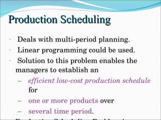
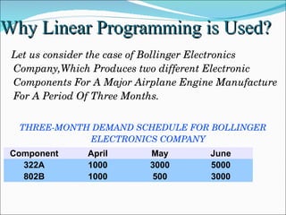
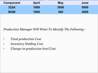
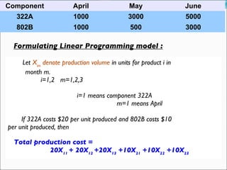
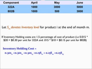
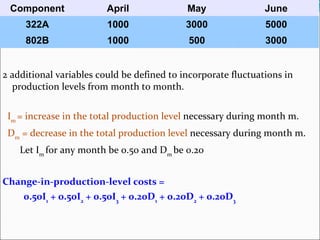
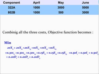
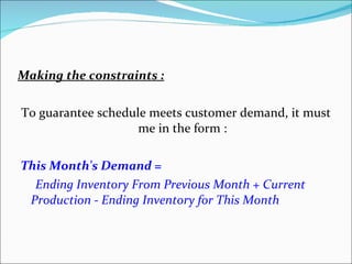
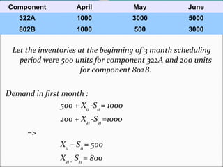
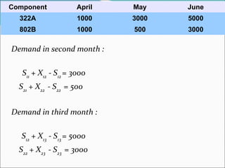
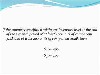
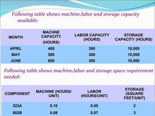
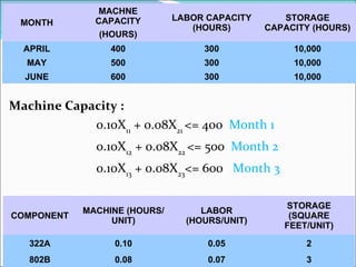
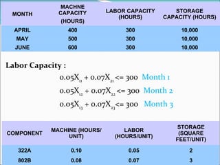
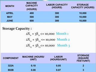
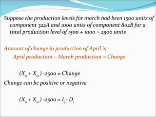
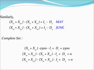
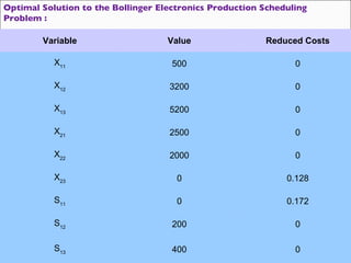
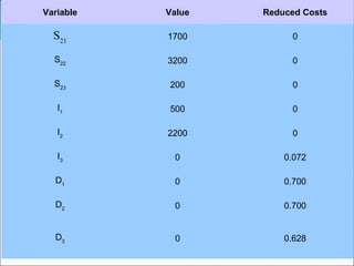
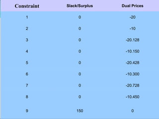
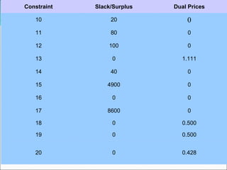
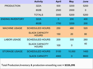
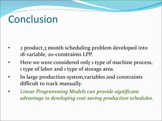
1. PRODUCTION SCHEDULING Meenu S Babu

2. Production Scheduling Deals with multi-period planning. Linear programming could be used. Solution to this problem enables the managers to establish an efficient low-cost production schedule for one or more products over several time period . Production Scheduling Problem is recursive.

3. Why Linear Programming is Used? Let us consider the case of Bollinger Electronics Company,Which Produces two different Electronic Components For A Major Airplane Engine Manufacture For A Period Of Three Months. THREE-MONTH DEMAND SCHEDULE FOR BOLLINGER ELECTRONICS COMPANY Component April May June 322A 1000 3000 5000 802B 1000 500 3000

4. Production Manager Will Want To Identify The Following : Total production Cost Inventory Holding Cost Change-in-production-level Cost Component April May June 322A 1000 3000 5000 802B 1000 500 3000

5. Formulating Linear Programming model : Let X im denote production volume in units for product i in month m. i=1,2 m=1,2,3 i=1 means component 322A m=1 means April If 322A costs $20 per unit produced and 802B costs $10 per unit produced, then Total production cost = 20X 11 + 20X 12 +20X 13 +10X 21 +10X 22 +10X 23 Component April May June 322A 1000 3000 5000 802B 1000 500 3000

6. Let S im denotes Inventory level for product i at the end of month m. If Inventory Holding costa are 1.5 percentage of cost of product (i.e 0.015 * $20 = $0.30 per unit for 322A and .015 * $10 = $0.15 per unit for 802B) Inventory Holding Cost = 0.30s 11 +0.30s 12 +0.30s 13 +0.15S 21 + 0.15S 22 +0.15S 23 Component April May June 322A 1000 3000 5000 802B 1000 500 3000

7. 2 additional variables could be defined to incorporate fluctuations in production levels from month to month. I m = increase in the total production level necessary during month m. D m = decrease in the total production level necessary during month m. Let I m for any month be 0.50 and D m be 0.20 Change-in-production-level costs = 0.50I 1 + 0.50I 2 + 0.50I 3 + 0.20D 1 + 0.20D 2 + 0.20D 3 Component April May June 322A 1000 3000 5000 802B 1000 500 3000

8. Combinig all the three costs, Objective function becomes : Min 20X 11 + 20X 12 +20X 13 +10X 21 +10X 22 +10X 23 +0.30s 11 +0.30s 12 +0.30s 13 +0.15S 21 + 0.15S 22 +0.15S 23 +0.50I 1 + 0.50I 2 + 0.50I 3 + 0.20D 1 + 0.20D 2 + 0.20D 3 Component April May June 322A 1000 3000 5000 802B 1000 500 3000

9. Making the constraints : To guarantee schedule meets customer demand, it must me in the form : This Month's Demand = Ending Inventory From Previous Month + Current Production - Ending Inventory for This Month

10. Let the inventories at the beginning of 3 month scheduling period were 500 units for component 322A and 200 units for component 802B. Demand in first month : 500 + X 11 -S 11 = 1000 200 + X 21 -S 21 =1000 => X 11 – S 11 = 500 X 21 – S 21 = 800 Component April May June 322A 1000 3000 5000 802B 1000 500 3000

11. Demand in second month : S 11 + X 12 - S 12 = 3000 S 21 + X 22 - S 22 = 500 Demand in third month : S 12 + X 13 - S 13 = 5000 S 22 + X 23 - S 23 = 3000 Component April May June 322A 1000 3000 5000 802B 1000 500 3000

12. If the company specifies a minimum inventory level at the end of the 3 month period of at least 400 units of component 322A and at least 200 units of component 802B, then S 13 >= 400 S 23 >= 200

13. Following table shows machine,labor and storage capacity available: Following table shows machine,labor and storage space requirement needed: MONTH MACHNE CAPACITY (HOURS) LABOR CAPACITY (HOURS) STORAGE CAPACITY (HOURS) APRIL 400 300 10,000 MAY 500 300 10,000 JUNE 600 300 10,000 COMPONENT MACHINE (HOURS/UNIT) LABOR (HOURS/UNIT) STORAGE (SQUARE FEET/UNIT) 322A 0.10 0.05 2 802B 0.08 0.07 3

14. Machine Capacity : 0.10X 11 + 0.08X 21 <= 400 Month 1 0.10X 12 + 0.08X 22 <= 500 Month 2 0.10X 13 + 0.08X 23 <= 600 Month 3 MONTH MACHNE CAPACITY (HOURS) LABOR CAPACITY (HOURS) STORAGE CAPACITY (HOURS) APRIL 400 300 10,000 MAY 500 300 10,000 JUNE 600 300 10,000 COMPONENT MACHINE (HOURS/UNIT) LABOR (HOURS/UNIT) STORAGE (SQUARE FEET/UNIT) 322A 0.10 0.05 2 802B 0.08 0.07 3

15. Labor Capacity : 0.05X 11 + 0.07X 21 <= 300 Month 1 0.05X 12 + 0.07X 22 <= 300 Month 2 0.05X 13 + 0.07X 23 <= 300 Month 3 MONTH MACHNE CAPACITY (HOURS) LABOR CAPACITY (HOURS) STORAGE CAPACITY (HOURS) APRIL 400 300 10,000 MAY 500 300 10,000 JUNE 600 300 10,000 COMPONENT MACHINE (HOURS/UNIT) LABOR (HOURS/UNIT) STORAGE (SQUARE FEET/UNIT) 322A 0.10 0.05 2 802B 0.08 0.07 3

16. Storage Capacity : 2X 11 + 3S 21 <= 10,000 Month 1 2X 12 + 3S 22 <= 10,000 Month 2 2X 13 + 3S 23 <= 10,000 Month 3 MONTH MACHNE CAPACITY (HOURS) LABOR CAPACITY (HOURS) STORAGE CAPACITY (HOURS) APRIL 400 300 10,000 MAY 500 300 10,000 JUNE 600 300 10,000 COMPONENT MACHINE (HOURS/UNIT) LABOR (HOURS/UNIT) STORAGE (SQUARE FEET/UNIT) 322A 0.10 0.05 2 802B 0.08 0.07 3

17. Suppose the production levels for march had been 1500 units of component 322A and 1000 units of component 802B for a total production level of 1500 + 1000 = 2500 units Amount of change in production of April is : April production – March production = Change (X 11 + X 21 ) -2500 = Change Change can be positive or negative (X 11 + X 21 ) -2500 = I 1 - D 1

18. Similarly, (X 12 + X 22 ) - (X 11 + X 21 ) = I 2 - D 2 MAY (X 13 + X 23 ) - (X 12 + X 22 ) = I 3 - D 3 JUNE Complete Set : (X 11 + X 21 ) -2500 - I 1 + D 1 = 2500 (X 12 + X 22 ) - (X 11 + X 21 ) - I 2 + D 2 = 0 (X 13 + X 23 ) - (X 12 + X 22 ) - I 3 + D 3 = 0

19. Optimal Solution to the Bollinger Electronics Production Scheduling Problem : Variable Value Reduced Costs X 11 500 0 X 12 3200 0 X 13 5200 0 X 21 2500 0 X 22 2000 0 X 23 0 0.128 S 11 0 0.172 S 12 200 0 S 13 400 0

20. Variable Value Reduced Costs S 21 1700 0 S 22 3200 0 S 23 200 0 I 1 500 0 I 2 2200 0 I 3 0 0.072 D 1 0 0.700 D 2 0 0.700 D 3 0 0.628

21. Constraint Slack/Surplus Dual Prices 1 0 -20 2 0 -10 3 0 -20.128 4 0 -10.150 5 0 -20.428 6 0 -10.300 7 0 -20.728 8 0 -10.450 9 150 0

22. Constraint Slack/Surplus Dual Prices 10 20 0 11 80 0 12 100 0 13 0 1.111 14 40 0 15 4900 0 16 0 0 17 8600 0 18 0 0.500 19 0 0.500 20 0 0.428

23. Total Production,Inventory & production-smoothing cost = $225,295 Activity April May June PRODUCTION 322A 500 3200 5200 802B 2500 2000 0 TOTALS 3000 5200 5200 ENDING INVENTORY 322A 0 200 400 802B 1700 3200 200 MACHINE USAGE SCHEDULED HOURS 250 480 520 SLACK CAPACITY HOURS 150 20 80 LABOR USAGE SCHEDULED HOURS 200 300 260 SLACK CAPACITY HOURS 100 0 40 STORAGE USAGE SCHEDULED HOURS 5100 10,000 1400 SLACK CAPACITY 4900 0 8600

24. Conclusion 2 product,3 month scheduling problem developed into 18-variable, 20-constraints LPP. Here we were considered only 1 type of machine process, 1 type of labor and 1 type of storage area. In large production system,variables and constraints difficult to track manually. Linear Programming Models can provide significant advantage in developing cost saving production schedules.