1. A random variable (RV) is a function that maps outcomes of a random phenomenon to numerical values. For a function X to be an RV, the set P(x) = {ω: X(ω) ≤ x} must be an event with a well-defined probability P for any x. 2. Conditional probability P(A|B) is the probability of event A occurring given that event B has occurred. It is defined as P(A ∩ B)/P(B). 3. The law of total probability states that for mutually exclusive and exhaustive events B1, B2, ..., the probability of event A is the sum of the probabilities of A given each Bi multiplied by

1. Applied Probability
Concepts & Examples
Johar M. Ashfaque
1 What is a Random Variable?
Let X be a function from the sample space Ω into the set of reals R. In order for X to be RV, some
extra requirements are needed. What are they?
The necessary and sufficient condition is: for each x ∈ R and ω ∈ Ω (an element in the set of all the
possible outcomes for the named event),
P(x) := {ω ∈ Ω : X(ω) ≤ x}
must be an event such that the probability P ∈ R≥0 that is the probability of the event taking place is
well-defined on P(x).
The point here is that for any function X : Ω → R, the set P(x) is not necessarily an event (in this case,
such an X is not a RV). Only for that function X which guarantees P(x) as an event for any x ∈ R, then
X is a RV.
There are two types of random variables: discrete and continuous. Where discrete random variables can
only take particular values or specified values in R, continuous random variables can take any value in
R.
A random variable has either an associated probability distribution (discrete random variable) or prob-
ability density function (continuous random variable).
1.1 Summary
Ω: The Sample Space (the set of all outcomes for the named event).
ω: An element of the sample space.
R: The set of real numbers.
X: A random variable if and only if for each x ∈ R and ω ∈ Ω
P(x) := {ω ∈ Ω : X(ω) ≤ x}
is an event with probability P ∈ R≥0 defined on P(x).
2 What is Conditional Probability?
Given any two events A and B which are not independent, the probability of event A taking place given
that event B has already taken place is defined by
P(A|B) =
P(A ∩ B)
P(B)
, P(B) > 0.
That is the probability of event A given that event B has already taken place is defined as the probability
of both event A and event B taking place divided by the probability of event B taking place.
If event A and event B are two independent events then
P(A ∩ B) = P(A)P(B)
1

2. and
P(A|B) = P(A).
This can be interpreted as the definition of independence.
3 The Law of Total Probability
Let ∪∞
i=1Bi be i mutually exclusive events. If ∪∞
i=1Bi = Ω where Ω is the sample space and for any i = j
Bi ∩ Bj = ∅
that is Bi and Bj are disjoint then
P(A) =
∞
i=1
P(Bi)P(A|Bi).
4 Conditional Probability: The Discrete Case
Suppose that X and Y are discrete RVs. For any x, y ∈ R consider the events {X = x} and {Y = y}
with
P(Y = y) > 0.
Define the conditional probability mass function of X given that Y = y by
pX|Y (x|y) =
p(x, y)
pY (y)
.
4.1 Example
Suppose that the joint mass function p(x, y) of X and Y is
p(1, 1) = 0.5, p(1, 2) = 0.1, p(2, 1) = 0.1, p(2, 2) = 0.3.
Let us calculate pX|Y (x|Y = 1).
To begin with let us compute pY (1) which is
pY (1) =
x
p(x, 1) = p(1, 1) + p(2, 1) = 0.6.
Now we can compute pX|Y (1|1) and pX|Y (2|1) very easily which can be found to be
pX|Y (1|1) =
5
6
and
pX|Y (2|1) =
1
6
.
5 Conditional Probability: The Continuous Case
Suppose that X and Y are continuous RVs. For any x, y ∈ R consider the events {X = x} and {Y = y}
with
P(Y = y) > 0.
2

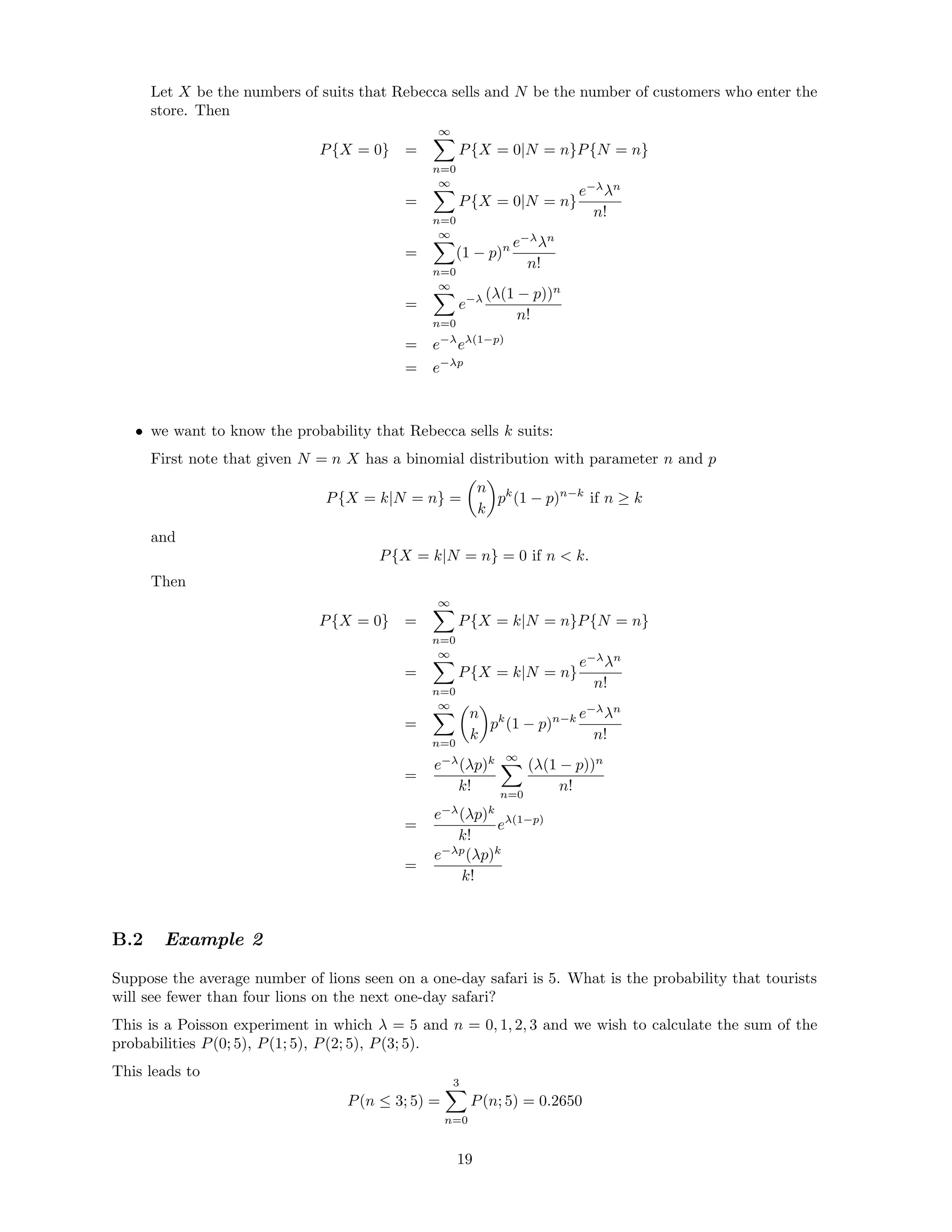
3. Define the conditional probability mass function of X given that Y = y by
fX|Y (x|y) =
f(x, y)
fY (y)
=
f(x, y)
∞
−∞
f(x, y)dx
and the associated conditional expectation is given by
E(X|Y = y) =
∞
−∞
xfX|Y (x|y)dx.
5.1 Example 1
Suppose the joint density of X and Y is given by
f(x, y) =
6xy(2 − x − y), 0 < x < 1, 0 < y < 1
0, otherwise.
Let us compute the conditional expectation of X given Y = y where 0 < y < 1.
If y ∈ (0, 1) we have for x ∈ (0, 1) that
fX|Y (x|y) =
f(x, y)
fY (y)
=
f(x, y)
∞
−∞
f(x, y)dx
=
6xy(2 − x − y)
1
0
6xy(2 − x − y)dx
=
6xy(2 − x − y)
4 − 3y
Then
E(X|Y = y) =
5 − 4y
8 − 6y
where y ∈ (0, 1).
5.2 Example 2
Consider the triangle in the plane R whose vertices are (0, 0), (0, 1) and (1, 0).
Let X and Y be continuous random variables for which the joint density is given by
f(x, y) =
2, 0 ≤ x ≤ 1, 0 ≤ y ≤ 1, x + y ≤ 1
0, otherwise.
Let us compute the conditional expectation of X given Y = y where 0 ≤ y ≤ 1. 0 ≤ y ≤ 1 tells us that
x ∈ [0, 1 − y] and so
fX|Y (x|y) =
2
1−y
0
2dx
=
1
1 − y
. Then
E(X|Y = y) =
1−y
0
x(1 − y)−1
dx =
1 − y
2
.
6 Discrete-Time Markov Chains & Transition Matrix
Let X1, X2,..., be independent RVs each taking values -1 and 1 with probabilities q = 1 − p and p where
p ∈ (0, 1).
Define the random walk
Sn = a +
n
i=1
Xi
by the position of the movement after n steps having started at S0 = a (in most cases a = 0).
For p = 1
2 , q = 1 − p = 1
2 and so we would have a symmetric random walk.
3

4. 6.1 Example: The Gambler’s Ruin
A man is saving to buy a BMW at a cost of N units of money. He stars with a (0 ≤ a ≤ N) units and
tries to win the remainder by a gamble.
He flips a fair coin repeatedly; if its heads his friend pays him one unit; for tails, he pays his friend one
unit. He keeps playing this game until either he runs out of money or he wins enough to buy.
This is an example of a symmetric random walk.
6.2 Random Stochastic Process
A random stochastic process is a group of random variables
{Xt : t ∈ T}
indexed by some set T ⊂ R where T can be be thought of as time.
If T ⊂ R is a discrete set, we speak of discrete time process {Xt}, t ∈ T.
If T happens to be continuous we speak of a continuous time process {Xt}, t ∈ T.
If the state space S of this process is finite then {Xt} is called a chain.
6.3 Discrete Time Markov Chain (DTMC)
{Xn} is a DTMC if it satisfies for all n
P{Xn+1 = in+1 X0 = i0, ..., Xn−1 = in−1, Xn = in}
= P{Xn+1 = in+1 Xn = in}
holds for arbitrary ik ∈ S for k = 0, 1, ..., n + 1, n ≥ 1. This means that the probability of any future
behaviour of the process when its present state is known is not altered by the additional knowledge of its
past behaviour. This is the Markovian property.
6.4 Example: Random Walk on the Cube
Let S = {(0, 0, 0), (0, 0, 1), (0, 1, 0), (0, 1, 1), (1, 0, 0), (1, 0, 1), (1, 1, 0), (1, 1, 1)} where each state represents
one corner of a cube in the obvious way in R3
:
(0, 1, 1) //
(1, 1, 1)
(0, 1, 0) //
(1, 1, 0)
(0, 0, 1) // (1, 0, 1)
(0, 0, 0) // (1, 0, 0)
We wish to write down the transition matrix of the Markov chain in which from any corner independently
of the past the next transition is equally likely to be to any of the three adjacent corners with probability
4

5. 1
3 .












(0, 0, 0) (0, 0, 1) (0, 1, 0) (0, 1, 1) (1, 0, 0) (1, 0, 1) (1, 1, 0) (1, 1, 1)
(0, 0, 0) 0 1/3 1/3 0 1/3 0 0 0
(0, 0, 1) 1/3 0 0 1/3 0 1/3 0 0
(0, 1, 0) 1/3 0 0 1/3 0 0 1/3 0
(0, 1, 1) 0 1/3 1/3 0 0 0 0 1/3
(1, 0, 0) 1/3 0 0 0 0 1/3 1/3 0
(1, 0, 1) 0 1/3 0 0 1/3 0 0 1/3
(1, 1, 0) 0 0 1/3 0 1/3 0 0 1/3
(1, 1, 1) 0 0 0 1/3 0 1/3 1/3 0












6.5 Another Example
Consider the Markov chain with three states S = {1, 2, 3} with
P =






1
2
1
4
1
4
1
3 0 2
3
1
2
1
2 0






then the state transition diagram for this chain is as shown below:
Figure 1: The State Transition Diagram
Furthermore, given
P(X1 = 1) = P(X1 = 2) =
1
4
we can find P(X1 = 3, X2 = 2, X3 = 1). Firstly, we will have to compute P(X1 = 3). We proceed as
follows
P(X1 = 3) = 1 − P(X1 = 1) − P(X1 = 2) = 1 −
1
4
−
1
4
=
1
2
.
5

6. Then
P(X1 = 3, X2 = 2, X3 = 1) = P(X1 = 3) · p3,2 · p2,1 =
1
12
.
7 Regular Transition Matrices
A transition matrix is regular if some power of the transition matrix contains all positive entries.
For example
A =


0.75 0.25 0
0 0.5 0.5
0.6 0.4 0


which squares to
A2
=


0.5625 0.3125 0.125
0.3 0.45 0.25
0.45 0.35 0.2


since all the entries in A2
are positive, matrix A is regular. But
B =


0.5 0 0.5
0 1 0
0 0 1


is not regular since
B2
=


0.25 0 0.75
0 1 0
0 0 1


and using the fact that if zeros occur in the identical places in both B and B2
than for higher power they
will appear in the same places. So no power of matrix B contains all positive entries.
8 Absorbing Markov Chains
State i of a Markov chain is an absorbing state if pii = 1.
A Markov chain is an absorbing chain if
• the chain has at least one absorbing state
• it is possible to go from any non-absorbing state to an absorbing state.
For example 

1 0 0
0.3 0.5 0.2
0 0 1


where p11 = 3 = p33 and we deduce that state 1 and state 3 are absorbing states. This is an example
of a Markov chain that is an absorbing chain since state 2 is non-absorbing and it is possible to go
from state 2 to state 1 and state 3.
However, 



0.6 0 0.4 0
0 1 0 0
0.9 0 0.1 0
0 0 0 1




is a Markov chain that is non-absorbing.
6

7. 9 Steady-State Distribution
We wish to find the steady state distribution for the following chain
Figure 2: The State Transition Diagram
we find
1
2
π1 +
1
3
π2 +
1
2
π3 = π1
1
4
π1 +
1
2
π3 = π2
1
4
π1 +
2
3
π2 = π3
π1 + π2 + π3 = 1
from which we deduce that
π3 =
10
9
π2 =
5
8
π1
and
π1 =
16
9
π2
giving
π1 =
16
35
π2 =
9
35
π3 =
10
35
.
7

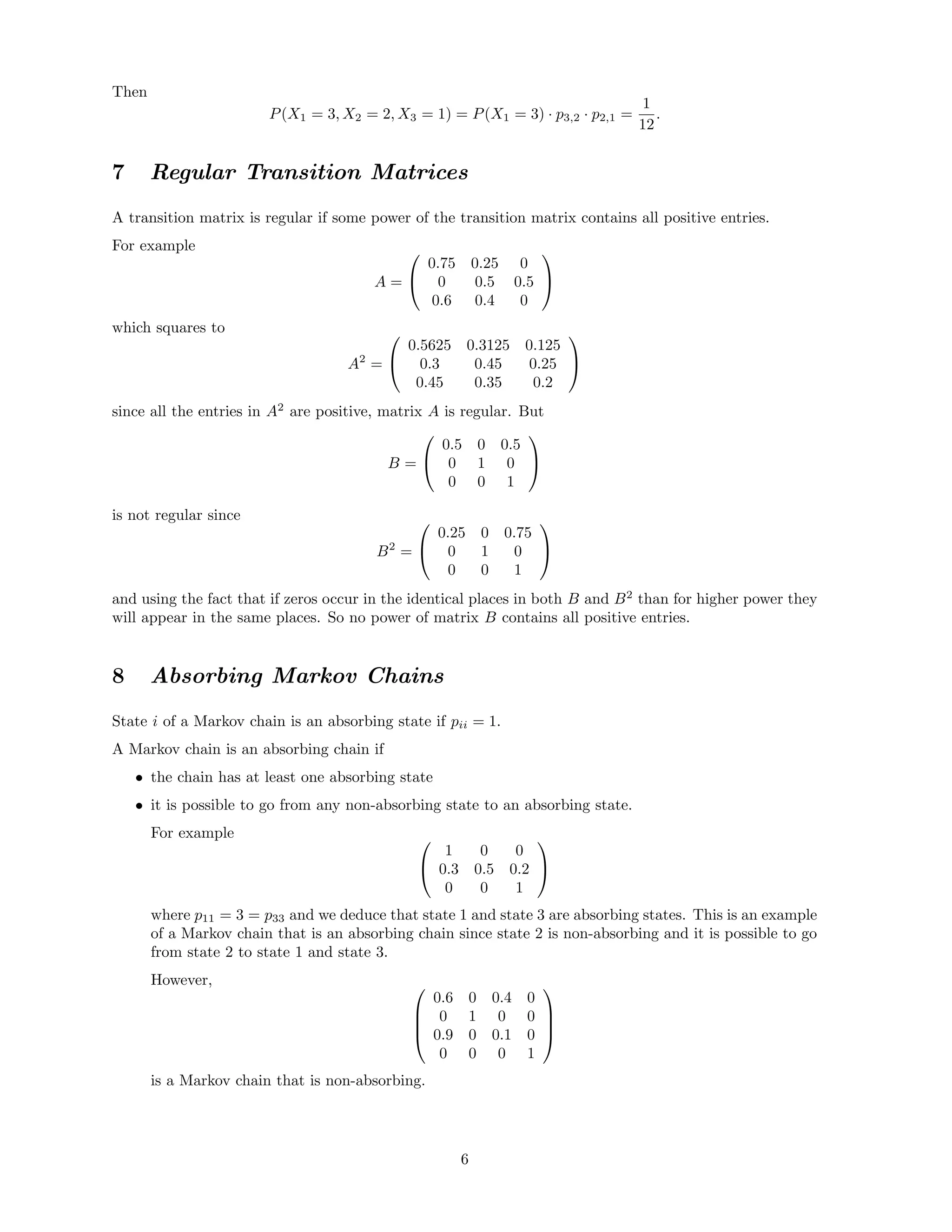
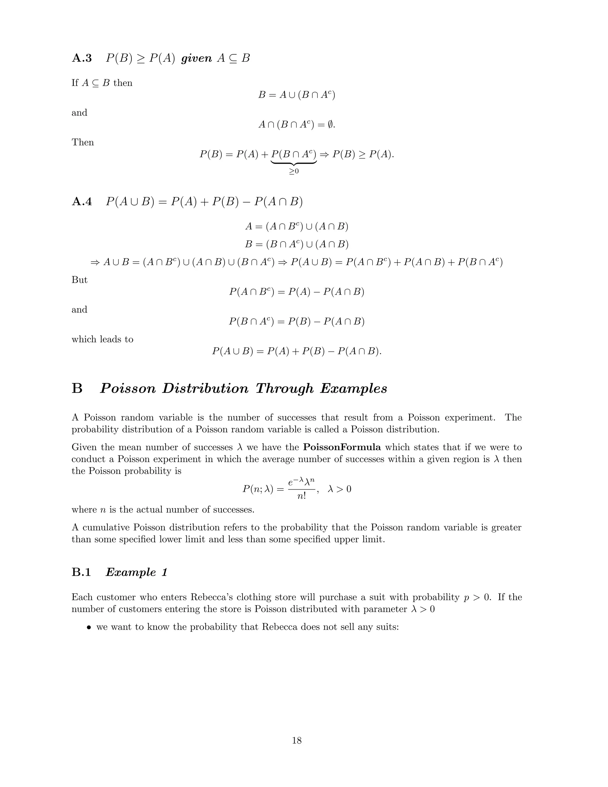
8. 10 More Examples of DTMC
A mobile robot randomly moves along a circular path divided into three sectors. At every sampling instant
the robot with probability p to move clockwise and with probability 1 − p to move counter-clockwise.
During the sampling interval the robot accomplishes the length of a sector.
• Define a discrete Markov chain for the random walk of the robot.
• Study the stationary probability that the robot is localized in each sector for p ∈ [0, 1].
State X = sector occupied by the robot ∈ {1, 2, 3}. The transition matrix reads


0 p 1 − p
1 − p 0 p
p 1 − p 0


For p = 0 we have
8

9. Each state of the Markov chain is periodic with period 3. Therefore, stationary probabilities do not exist.
p = 1 case is similar to the p = 0 case.
If p ∈ (0, 1) the Markov chain is irreducible aperiodic and finite. Therefore, the stationary-state proba-
bilities exist.
The unique steady state probability vector is given by
π = (
1
3
,
1
3
,
1
3
)
which is the solution of the system of equations
π = πP
3
i=1
πi = 1
11 Reversible Markov Chains
A Markov chain is with stationary distribution π is reversible if and only if
πipij = πjpji
for all states i and j.
11.1 Random Walk on a Graph
Recall that a graph is a collection of vertices where the ith vertex vi is directly joined by at most one
edge each to di other vertices (called its neighbour).
If
σ =
i
di ∞
then a random walk on the vertices of the graph simply goes to any one of the neighbours of vi with
equal probability 1
di
. Such a walk is reversible. To see this note that the detailed balance equations take
the form
πi
di
=
πj
dj
for neighbours i and j and the solution such that
i
πi = 1
is obviously
πi =
di
σ
.
11.2 The Ehrenfest Model
M balls distributed in two urns. Each time, pick a ball at random, move it from one urn to the other
one. Let Xn be the number of balls in urn 1. Prove that the chain has a reversible distribution.
The non-zero transition probabilities are
pi,i−1 =
i
M
pi,i+1 =
M − i
M
9

10. We are seeking solutions to
πipi,i+1 = πi+1pi+1,i ⇒ πi
M − i
M
= πi+1
i + 1
M
leading to
πi
π0
=
(M − i − 1)(M − i)...M
i(i − 1)...1
=
M
i
.
Note.
i
πi = 1 = π0
i
M
i
⇒ π0 =
1
2m
.
Note. Using
pi,i−1 =
i
M
and i → i + 1 arrive at
pi+1,i =
i + 1
M
.
The chain is irreducible and periodic.
12 Continuous-Time Markov Chains
We will consider a random process
{X(t), t ∈ [0, ∞)}.
We assume that we have a countable state space
S ⊂ {0, 1, 2, ...}.
If X(0) = i, then X(t) stays in state i for a random amount of time say T1 where T1 is a continuous
random variable. At time T1, the process jumps to a new state j and will spend a random amount of
time T2 in that state and so on. The random variables T1, T2, ... follow an exponential distribution. The
probability of going from state i to state j is denoted pij.
In particular, suppose that at time t, we know that X(t) = i. To make any prediction about the future,
it should not matter how long the process spends in each state and therefore must have a ”memoryless”
property. The exponential distribution is the only continuous distribution with the ”memoryless” prop-
erty. Thus, the time that a continuous-time Markov chain spends in state i known as the holding time
will have an exponential distribution: eλi
where λi is a non-negative real number. We further assume
that the λis are bounded that is there exists a real number M ∞ such that λi M for all i ∈ S.
A continuous-time Markov chain has two components. First is the discrete-time Markov chain known as
the jump chain or an embedded Markov chain which give the transition probabilities pij. The second is,
for each state, there is a holding time parameter λi that controls the time spent in each state.
12.1 An Example
Consider a Markov chain with two states S = {0, 1}. Assume the holding time parameters are given by
λ0 = λ1 = λ 0. That is, the time that the chain spends in each state before going to the other state
has eλ
distribution.
• Draw the state diagram of the embedded (jump) chain.
• Find the transition matrix P(t). You may find the following identities useful
sinh(x) =
ex
− e−x
2
=
∞
n=0
x2n+1
(2n + 1)!
cosh(x) =
ex
+ e−x
2
=
∞
n=0
x2n
(2n)!
10

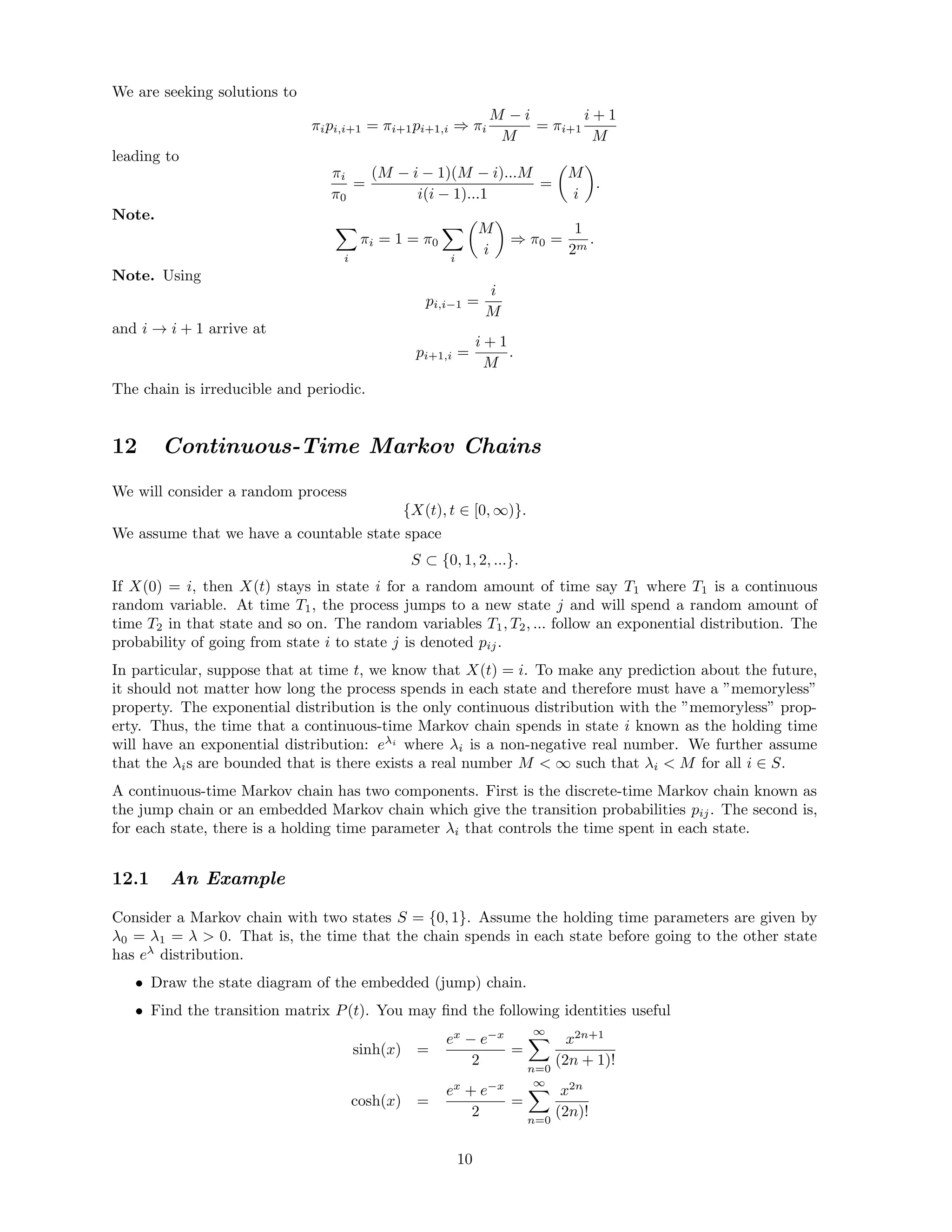
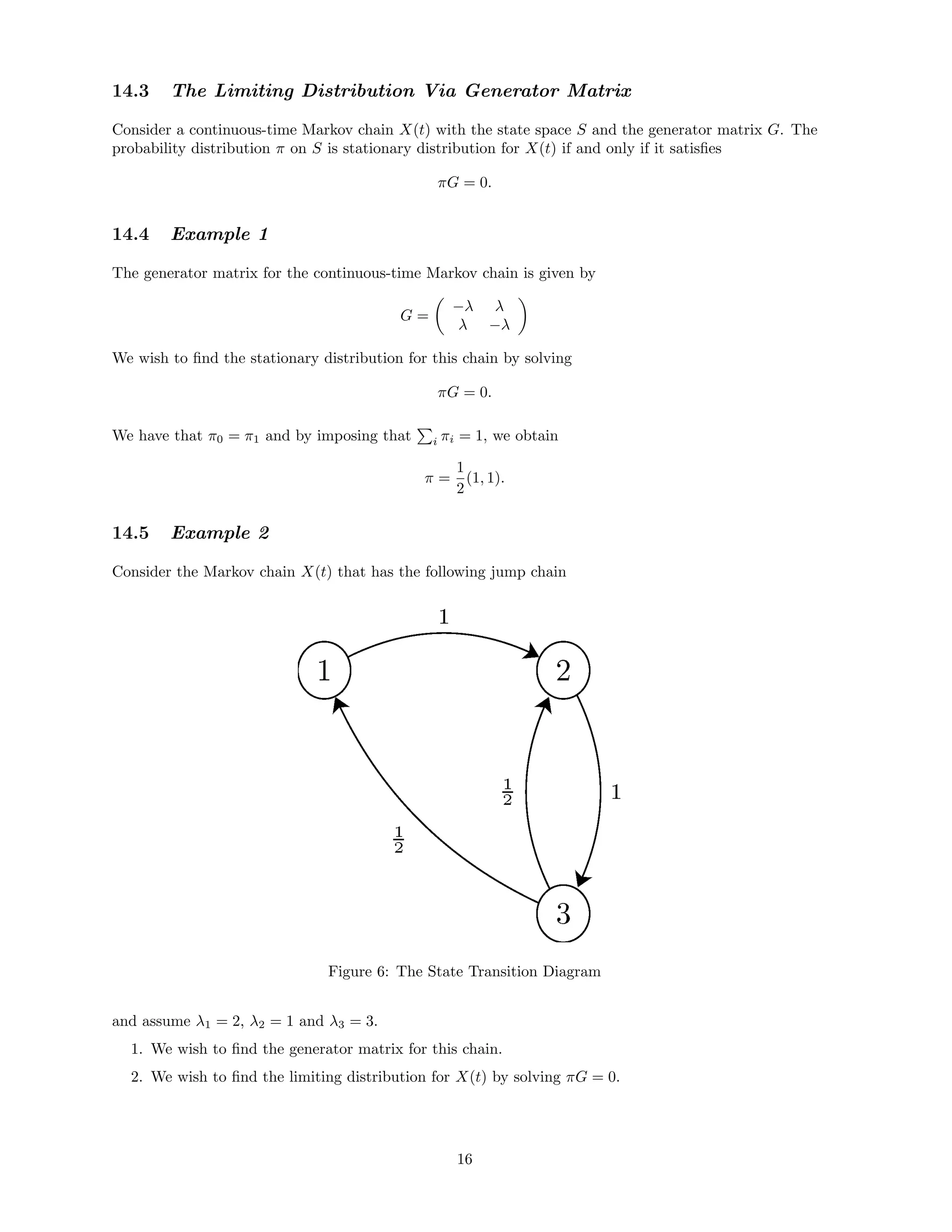
11. 12.2 The Solution: Part 1
There are two states in the chain and none of them are absorbing as λ0 = λ1 = λ 0. The jump chain
must therefore have the following transition matrix
P =
0 1
1 0
where the state-transition diagram of the embedded (jump) chain is
Figure 3: The State Transition Diagram
12.3 The Solution: Part 2
The Markov chain has a simple structure. Lets find P00(t). By definition
P00(t) = P(X(t) = 0|X(0) = 0), ∀t ∈ [0, ∞).
Assuming that X(0) = 0, X(t) will be 0 if and only if we have an even number of transitions in the time
interval [0, t]. The time between each transition is an eλ
random variable. Therefore, the transitions
occur according to a Poisson process with parameter λ.
We find
P00(t) =
∞
n=0
e−λt (λt)2n
(2n)!
= e−λt
∞
n=0
(λt)2n
(2n)!
= e−λt eλt
+ e−λt
2
=
1
2
+
1
2
e−2λt
P01(t) = 1 − P00(t) =
1
2
−
1
2
e−2λt
.
11

12. P11(t) = P00(t).
P10(t) = P01(t).
Therefore, the transition matrix for any t ≥ 0 is given by
P(t) =


1
2 + 1
2 e−2λt 1
2 − 1
2 e−2λt
1
2 − 1
2 e−2λt 1
2 + 1
2 e−2λt


Letting t go to infinity, the transition matrix reads
lim
t→∞
P(t) =


1
2
1
2
1
2
1
2


12.4 CTMC Transition Matrix: Properties
The transition matrix satisfies the following properties:
1. P(0) is equal to the identity matrix, P(0) = I;
2. The rows of the transition matrix must sum to 1
j∈S
pij(t) = 1, ∀t ≥ 0;
3. For all s, t ≥ 0,
P(s + t) = P(s)P(t).
13 CTMC: Limiting Distribution Examples
13.1 Example 1
Consider a continuous-time Markov chain X(t) that has the jump chain
Figure 4: The State Transition Diagram
12

13. Assume the holding parameters are given by
λ1 = 2, λ2 = 1, λ3 = 3.
We wish to find the limiting distribution of X(t).
First notice that the chain is irreducible. The transition matrix of the jump chain reads
P(t) =


0 1 0
0 0 1
1
2
1
2 0


the stationary distribution for the jump chain being
˜π =
1
5
(1, 2, 2).
This is obtained by solving the following system of equations
π3 = 2π1
π2 = 2π1
π2 = π3
3
i=1
πi = 1
The limiting distribution of X(t) can then be obtained by using
πj =
˜πj
λj
k∈S
˜πk
λk
.
Hence, we conclude that
π =
1
19
(3, 12, 4)
is the limiting distribution of X(t).
13.2 Example 2
Consider a continuous-time Markov chain X(t) that has the jump chain
13

14. Figure 5: The State Transition Diagram
Assume the holding parameters are given by
λ1 = 2, λ2 = 3, λ3 = 4.
We wish to find the limiting distribution of X(t).
First notice that the chain is irreducible. The transition matrix of the jump chain reads
P(t) =


0 1
2
1
2
0 1
3
2
3
1
2 0 1
2


the stationary distribution for the jump chain being
˜π =
1
15
(4, 3, 8).
The limiting distribution of X(t) can then be obtained by using
πj =
˜πj
λj
k∈S
˜πk
λk
which gives
π =
1
5
(2, 1, 2)
as the limiting distribution of X(t).
14

15. 14 Continuous-Time Markov Chains: The Generator Matrix
For a continuous-time Markov chain, define the generator matrix G as a transition matrix whose (i, j)-th
entry is given by
gij =
λipij if i = j
−λi if i = j
14.1 Example
A chain with two states S = {0, 1} and λ0 = λ1 = λ 0. We found that the transition matrix for any
t ≥ 0 is given by
P(t) =


1
2 + 1
2 e−2λt 1
2 − 1
2 e−2λt
1
2 − 1
2 e−2λt 1
2 + 1
2 e−2λt

 .
We wish
1. To find the generator matrix G
2. Show that for any t ≥ 0
P (t) = P(t)G = GP(t).
By definition
g00 = −λ0 = −λ
g11 = −λ1 = −λ
g01 = λ0p01
= λ
g10 = λ1p10
= λ
Thus, the generator matrix is given by
G =
−λ λ
λ −λ
To show that for any t ≥ 0
P (t) = P(t)G = GP(t)
we note that
P (t) =
−λe−2λt
λe−2λt
λe−2λt
−λe−2λt
We also have that
P(t)G =
−λe−2λt
λe−2λt
λe−2λt
−λe−2λt = GP(t).
14.2 The Forward and Backward Equations
• The forward equations state that
P (t) = P(t)G
• The backward equations state that
P (t) = GP(t)
15

16. 14.3 The Limiting Distribution Via Generator Matrix
Consider a continuous-time Markov chain X(t) with the state space S and the generator matrix G. The
probability distribution π on S is stationary distribution for X(t) if and only if it satisfies
πG = 0.
14.4 Example 1
The generator matrix for the continuous-time Markov chain is given by
G =
−λ λ
λ −λ
We wish to find the stationary distribution for this chain by solving
πG = 0.
We have that π0 = π1 and by imposing that i πi = 1, we obtain
π =
1
2
(1, 1).
14.5 Example 2
Consider the Markov chain X(t) that has the following jump chain
Figure 6: The State Transition Diagram
and assume λ1 = 2, λ2 = 1 and λ3 = 3.
1. We wish to find the generator matrix for this chain.
2. We wish to find the limiting distribution for X(t) by solving πG = 0.
16

17. The jump chain is irreducible and the transition matrix of the jump chain is given by
P(t) =


0 1 0
0 0 1
1
2
1
2 0


and by definition, we have the generator matrix G with entries
G =


−2 2 0
0 −1 1
3
2
3
2 −3

 .
Now by solving
πG = 0
we will be able to find the limiting distribution. We obtain the following system of equations
−2π1 +
3
2
π3 = 0
2π1 − π2 +
3
2
π3 = 0
π2 − 3π3 = 0
Then imposing i πi = 1, we find that
π =
1
19
(3, 12, 4)
is the limiting distribution of X(t).
A Axioms of Probability
Given
• P(Ω) = 1
• 0 ≤ P(A) ≤ 1 for any event A ⊆ Ω
• if A1, ..., An are events and Ai ∩ Aj = ∅ for all i = j then
PP(A1 ∪ A2 ∪ ... ∪ An) =
n
i=1
P(Ai).
A.1 P(Ac
) = 1 − P(A)
A and Ac
are disjoint that is A ∩ Ac
= ∅.
A ∪ Ac
= Ω ⇒ P(A) + P(Ac
) = P(Σ) = 1
from which follows that
P(Ac
) = 1 − P(A).
A.2 P(∅) = 0
P(∅) = P(Ωc
) = 1 − P(Ω) = 1 − 1 = 0.
17

18. A.3 P(B) ≥ P(A) given A ⊆ B
If A ⊆ B then
B = A ∪ (B ∩ Ac
)
and
A ∩ (B ∩ Ac
) = ∅.
Then
P(B) = P(A) + P(B ∩ Ac
)
≥0
⇒ P(B) ≥ P(A).
A.4 P(A ∪ B) = P(A) + P(B) − P(A ∩ B)
A = (A ∩ Bc
) ∪ (A ∩ B)
B = (B ∩ Ac
) ∪ (A ∩ B)
⇒ A ∪ B = (A ∩ Bc
) ∪ (A ∩ B) ∪ (B ∩ Ac
) ⇒ P(A ∪ B) = P(A ∩ Bc
) + P(A ∩ B) + P(B ∩ Ac
)
But
P(A ∩ Bc
) = P(A) − P(A ∩ B)
and
P(B ∩ Ac
) = P(B) − P(A ∩ B)
which leads to
P(A ∪ B) = P(A) + P(B) − P(A ∩ B).
B Poisson Distribution Through Examples
A Poisson random variable is the number of successes that result from a Poisson experiment. The
probability distribution of a Poisson random variable is called a Poisson distribution.
Given the mean number of successes λ we have the PoissonFormula which states that if we were to
conduct a Poisson experiment in which the average number of successes within a given region is λ then
the Poisson probability is
P(n; λ) =
e−λ
λn
n!
, λ 0
where n is the actual number of successes.
A cumulative Poisson distribution refers to the probability that the Poisson random variable is greater
than some specified lower limit and less than some specified upper limit.
B.1 Example 1
Each customer who enters Rebecca’s clothing store will purchase a suit with probability p 0. If the
number of customers entering the store is Poisson distributed with parameter λ 0
• we want to know the probability that Rebecca does not sell any suits:
18

19. Let X be the numbers of suits that Rebecca sells and N be the number of customers who enter the
store. Then
P{X = 0} =
∞
n=0
P{X = 0|N = n}P{N = n}
=
∞
n=0
P{X = 0|N = n}
e−λ
λn
n!
=
∞
n=0
(1 − p)n e−λ
λn
n!
=
∞
n=0
e−λ (λ(1 − p))n
n!
= e−λ
eλ(1−p)
= e−λp
• we want to know the probability that Rebecca sells k suits:
First note that given N = n X has a binomial distribution with parameter n and p
P{X = k|N = n} =
n
k
pk
(1 − p)n−k
if n ≥ k
and
P{X = k|N = n} = 0 if n k.
Then
P{X = 0} =
∞
n=0
P{X = k|N = n}P{N = n}
=
∞
n=0
P{X = k|N = n}
e−λ
λn
n!
=
∞
n=0
n
k
pk
(1 − p)n−k e−λ
λn
n!
=
e−λ
(λp)k
k!
∞
n=0
(λ(1 − p))n
n!
=
e−λ
(λp)k
k!
eλ(1−p)
=
e−λp
(λp)k
k!
B.2 Example 2
Suppose the average number of lions seen on a one-day safari is 5. What is the probability that tourists
will see fewer than four lions on the next one-day safari?
This is a Poisson experiment in which λ = 5 and n = 0, 1, 2, 3 and we wish to calculate the sum of the
probabilities P(0; 5), P(1; 5), P(2; 5), P(3; 5).
This leads to
P(n ≤ 3; 5) =
3
n=0
P(n; 5) = 0.2650
19

20. B.3 Example 3
The number of baseball games rained out is a Poisson process with arrival rate of 5 per 30 days.
• We wish to find the probability that there are more than 5 rained out games in 15 days.
• We wish to find the probability that there are no rained out games in 7 days.
First note that
λ =
5
30
=
1
6
and the total number of rained out games in t days is Poisson( t
6 ). To find the probability that there are
more than 5 rained out games in 15 days reduces to
1 − P(n ≤ 5;
5
2
) = 0.042.
Similarly, the probability that there are no rained out games in 7 days is
e−7/6
= 0.311
20