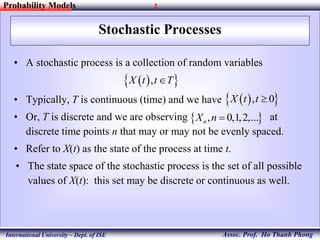
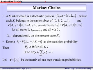
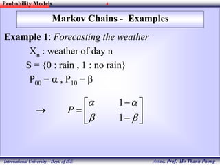
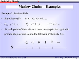
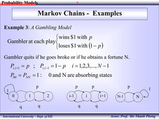
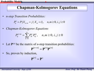
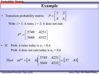
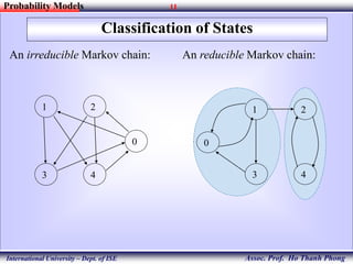
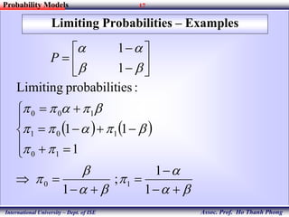
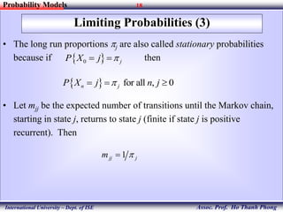
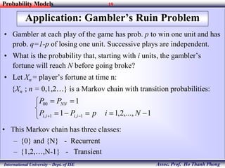
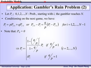
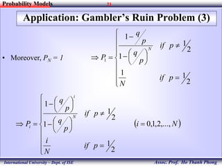
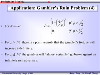
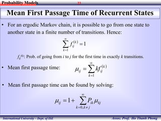
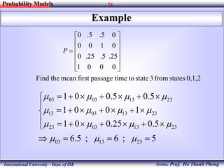
1
Assoc. Prof. Ho Thanh Phong
Probability Models
International University – Dept. of ISE
 Introduction Stochastic Processes.
 Markov Chains.
 Chapman-Kolmogorov Equations
 Classification of States
 Recurrence and Transience
 Limiting Probabilities
Markov Chains4
2
Assoc. Prof. Ho Thanh Phong
Probability Models
International University – Dept. of ISE
Stochastic Processes
• A stochastic process is a collection of random variables
• Typically, T is continuous (time) and we have
• Or, T is discrete and we are observing at
discrete time points n that may or may not be evenly spaced.
• Refer to X(t) as the state of the process at time t.
• The state space of the stochastic process is the set of all possible
values of X(t): this set may be discrete or continuous as well.
  ,X t t T
 , 0,1,2,...nX n 
  , 0X t t 
3
Assoc. Prof. Ho Thanh Phong
Probability Models
International University – Dept. of ISE
Markov Chains
• A Markov chain is a stochastic process , where
each Xn belongs to the same subset of {0, 1, 2, …}, and
for all states i0, i1,…, in-1 and all n  0 .
• Denote as the transition probability
Then
Let be the matrix of one-step transition probabilities.
 , 0,1,2,...nX n 
   1 1 1 1 1 0 0 1, ,..., ,n n n n n nP X j X i X i X i X i P X j X i          
 1ij n nP P X j X i  
ijP   P
nn XX statepresenton theonlydepends1
1,anyFor
,allfor0


jall
ij
ij
Pi
jiP
4
Assoc. Prof. Ho Thanh Phong
Probability Models
International University – Dept. of ISE
Markov Chains - Examples
Example 1: Forecasting the weather
Xn : weather of day n
S = {0 : rain , 1 : no rain}
P00 =  , P10 = 











1
1
P
5
Assoc. Prof. Ho Thanh Phong
Probability Models
International University – Dept. of ISE
Markov Chains - Examples
Example 2: Forecasting the weather
• If it rains for the past two days then it will rain tomorrow with probability
0.7
• If it rains today but not yesterday then it will rain tomorrow with
probability 0.5
• If it rains yesterday but not today then it will rain tomorrow with
probability 0.4
• If it has not rain in the past two days then it will rain tomorrow with
probability 0.2
States: 0: RR, 1: NR, 2: RN, 3: NN













8.02.0
6.04.0
05.05.
03.07.
P
6
Assoc. Prof. Ho Thanh Phong
Probability Models
International University – Dept. of ISE
Markov Chains - Examples
Example 3: Random Walks
• State Space (S): 0, ±1, ±2, ±3, ±4,….
• Pi, i + 1 = p ; Pi, i - 1 = 1 – p i = 0, 1, …
• At each point of time, either it takes one step to the right with
probability p, or one step to the left with probability 1-p.
S
-2 -1 0 1 2 ……
7
Assoc. Prof. Ho Thanh Phong
Probability Models
International University – Dept. of ISE
Markov Chains - Examples
Example 3: A Gambling Model
Gambler quits if he goes broke or if he obtains a fortune N.
 


 p
p
1with$1loses
with$1wins
playeachatGambler
statesabsorbingareNand0:1
1,...,3,2,11;
00
1,1,

 
NN
iiii
PP
NipPpP
0 1 2 i-1 i i+1 N-1 N
1 1
p p p p
q q q q
8
Assoc. Prof. Ho Thanh Phong
Probability Models
International University – Dept. of ISE
Chapman-Kolmogorov Equations
• n-step Transition Probabilities:
• Chapman-Kolmogorov Equations
• Let P(n) be the matrix of n-step transition probabilities:
• So, proven by induction,
{ | }, , 0, , 0n
ij n m mP P X j X i n m i j    
0
, , 0, , 0n m n m
ij ik kj
k
P P P n m i j



  
     n m n m
P P P
 n n
P P
9
Assoc. Prof. Ho Thanh Phong
Probability Models
International University – Dept. of ISE
Example
• Transition probability matrix: 






6.4.
3.7.
P
With: i = 1: it rains; i = 2: it does not rain







4332.5668.
4251.5749.4
P
• If: Prob. it rains today is α1 = 0.4
Prob. it does not rain today is α2 = 0.6
   43.57.
4332.5668.
4251.5749.
6.4.4






PThen 
10
Assoc. Prof. Ho Thanh Phong
Probability Models
International University – Dept. of ISE
Classification of States
• State j is accessible from state i if
• If j is accessible from i and i is accessible from j, we say that states i
and j communicate (i  j).
• Communication is a class property:
(i) State i communicates with itself, for all i  0
(ii) If i  j then j  i : communicate is commutative
(iii) If i  j and j  k, then i  k : communicate is transitive
• Therefore, communication divides the state space up into mutually
exclusive classes.
• If all the states communicate, the Markov chain is irreducible.
0 for some 0n
ijP n 
11
Assoc. Prof. Ho Thanh Phong
Probability Models
International University – Dept. of ISE
Classification of States
An irreducible Markov chain:
0
3 4
21
An reducible Markov chain:
0
3 4
21
12
Assoc. Prof. Ho Thanh Phong
Probability Models
International University – Dept. of ISE
Recurrence vs. Transience
• Let fi be the probability that, starting in state i, the process will ever
reenter state i. If fi = 1, the state is recurrent, otherwise it is transient.
– If state i is recurrent then, starting from state i, the process will reenter state i
infinitely often (w/prob. 1).
– If state i is transient then, starting in state i, the number of periods in which the
process is in state i has a geometric distribution with parameter 1 – fi.
• state i is recurrent if and transient if
• Recurrence (transience) is a class property: If i is recurrent
(transient) and i  j then j is recurrent (transient).
• A special case of a recurrent state is if Pii = 1 then i is absorbing.
1
n
iin
P


  1
n
iin
P


 
13
Assoc. Prof. Ho Thanh Phong
Probability Models
International University – Dept. of ISE
Recurrence vs. Transience (2)
• Not all states in a finite Markov chain can be transient.
• All states of a finite irreducible Markov chain are recurrent.
• If state i is recurrent and state i does not communicate with
state j, then
– when a process enters a recurrent class of states it can
never leave that class.
– A recurrent class is often called a closed class
0ijP
14
Assoc. Prof. Ho Thanh Phong
Probability Models
International University – Dept. of ISE
Examples
recurrentarestatesAll
0010
0010
0001
5.5.00












P
     transientrecurrentP 
















 4:Class;3,2,1,0:Classes
5.0025.25.
05.5.00
05.5.00
0005.5.
0005.5.
recurrentarestatesalli
0100
005.5.
1000
1000













 rreducibleP
15
Assoc. Prof. Ho Thanh Phong
Probability Models
International University – Dept. of ISE
Limiting Probabilities
• If whenever n is not divisible by d, and d is the largest
integer with this property, then state i is periodic with period d.
• If a state has period d = 1, then it is aperiodic.
• If state i is recurrent and if, starting in state i, the expected time until
the process returns to state i is finite, it is positive recurrent
(otherwise it is null recurrent).
• A positive recurrent, aperiodic state is called ergodic.
0n
iiP 
16
Assoc. Prof. Ho Thanh Phong
Probability Models
International University – Dept. of ISE
Limiting Probabilities (2)
Theorem:
• For an irreducible ergodic Markov chain, exists for all
j and is independent of i.
• Furthermore, pj is the unique nonnegative solution of
• The probability pj also equals the long run proportion of time that the
process is in state j.
lim n
j ij
n
Pp


0
0
, 0
1
j i ij
i
j
j
P jp p
p




 



17
Assoc. Prof. Ho Thanh Phong
Probability Models
International University – Dept. of ISE
Limiting Probabilities – Examples











1
1
P
   


p


p
pp
ppp
ppp













1
1
;
1
1
11
:iesprobabilitLimiting
10
10
101
100
18
Assoc. Prof. Ho Thanh Phong
Probability Models
International University – Dept. of ISE
Limiting Probabilities (3)
• The long run proportions pj are also called stationary probabilities
because if then
• Let mjj be the expected number of transitions until the Markov chain,
starting in state j, returns to state j (finite if state j is positive
recurrent). Then
 0 jP X j p 
  for all , 0n jP X j n jp  
1jj jm p
19
Assoc. Prof. Ho Thanh Phong
Probability Models
International University – Dept. of ISE
Application: Gambler’s Ruin Problem
• Gambler at each play of the game has prob. p to win one unit and has
prob. q=1-p of losing one unit. Successive plays are independent.
• What is the probability that, starting with i units, the gambler’s
fortune will reach N before going broke?
• Let Xn = player’s fortune at time n:
{Xn ; n = 0,1,2…} is a Markov chain with transition probabilities:





 1,...,2,11
1
1,1,
00
NipPP
PP
iiii
NN
• This Markov chain has three classes:
– {0} and {N} - Recurrent
– {1,2,…,N-1} - Transient
20
Assoc. Prof. Ho Thanh Phong
Probability Models
International University – Dept. of ISE
Application: Gambler’s Ruin Problem (2)
• Let Pi ; 0,1,2,...,N : Prob., starting with i, the gambler reaches N.
• Conditioning on the next game, we have:
  1,...,2,11111   NiforPP
p
q
PPorqPpPP iiiiiii
• Note that: P0 = 0
 Ni
p
qifiP
p
qifP
p
q
p
q
P
i
i ,...,2
1
1
1
1
1
1


















21
Assoc. Prof. Ho Thanh Phong
Probability Models
International University – Dept. of ISE
Application: Gambler’s Ruin Problem (3)
• Moreover, PN = 1


















2
11
2
1
1
1
1
pif
N
pif
p
q
p
q
P
N
 Ni
pif
N
i
pif
p
q
p
q
P
N
i
i ,...,2,1,0
2
1
2
1
1
1























22
Assoc. Prof. Ho Thanh Phong
Probability Models
International University – Dept. of ISE
Application: Gambler’s Ruin Problem (4)
• For N → ∞:












2
10
2
11
pif
pif
p
q
P
i
i
• For p > 1/2: there is a positive prob. that the gambler’s fortune will
increase indefinitely.
• For p ≤ 1/2: the gambler will “almost certainly” go broke against an
infinitely rich adversary.
23
Assoc. Prof. Ho Thanh Phong
Probability Models
International University – Dept. of ISE
Mean First Passage Time of Recurrent States
 
1
1


k
k
ijf
• For an ergodic Markov chain, it is possible to go from one state to
another state in a finite number of transitions. Hence:
fij
(k): Prob. of going from i to j for the first time in exactly k transitions.
• Mean first passage time:  




1k
k
ijij kf
• Mean first passage time can be found by solving:




jkk
kjikij P
,0
1 
24
Assoc. Prof. Ho Thanh Phong
Probability Models
International University – Dept. of ISE
Example
0,1,2statesfrom3statetotimepassagefirstmeantheFind
0001
25.5.25.0
0100
05.5.0












P
5;6;5.6
5.025.001
1001
5.05.001
231303
23130323
23130313
23130303














Chap 4 markov chains

  • 1.
    1 Assoc. Prof. HoThanh Phong Probability Models International University – Dept. of ISE  Introduction Stochastic Processes.  Markov Chains.  Chapman-Kolmogorov Equations  Classification of States  Recurrence and Transience  Limiting Probabilities Markov Chains4
  • 2.
    2 Assoc. Prof. HoThanh Phong Probability Models International University – Dept. of ISE Stochastic Processes • A stochastic process is a collection of random variables • Typically, T is continuous (time) and we have • Or, T is discrete and we are observing at discrete time points n that may or may not be evenly spaced. • Refer to X(t) as the state of the process at time t. • The state space of the stochastic process is the set of all possible values of X(t): this set may be discrete or continuous as well.   ,X t t T  , 0,1,2,...nX n    , 0X t t 
  • 3.
    3 Assoc. Prof. HoThanh Phong Probability Models International University – Dept. of ISE Markov Chains • A Markov chain is a stochastic process , where each Xn belongs to the same subset of {0, 1, 2, …}, and for all states i0, i1,…, in-1 and all n  0 . • Denote as the transition probability Then Let be the matrix of one-step transition probabilities.  , 0,1,2,...nX n     1 1 1 1 1 0 0 1, ,..., ,n n n n n nP X j X i X i X i X i P X j X i            1ij n nP P X j X i   ijP   P nn XX statepresenton theonlydepends1 1,anyFor ,allfor0   jall ij ij Pi jiP
  • 4.
    4 Assoc. Prof. HoThanh Phong Probability Models International University – Dept. of ISE Markov Chains - Examples Example 1: Forecasting the weather Xn : weather of day n S = {0 : rain , 1 : no rain} P00 =  , P10 =             1 1 P
  • 5.
    5 Assoc. Prof. HoThanh Phong Probability Models International University – Dept. of ISE Markov Chains - Examples Example 2: Forecasting the weather • If it rains for the past two days then it will rain tomorrow with probability 0.7 • If it rains today but not yesterday then it will rain tomorrow with probability 0.5 • If it rains yesterday but not today then it will rain tomorrow with probability 0.4 • If it has not rain in the past two days then it will rain tomorrow with probability 0.2 States: 0: RR, 1: NR, 2: RN, 3: NN              8.02.0 6.04.0 05.05. 03.07. P
  • 6.
    6 Assoc. Prof. HoThanh Phong Probability Models International University – Dept. of ISE Markov Chains - Examples Example 3: Random Walks • State Space (S): 0, ±1, ±2, ±3, ±4,…. • Pi, i + 1 = p ; Pi, i - 1 = 1 – p i = 0, 1, … • At each point of time, either it takes one step to the right with probability p, or one step to the left with probability 1-p. S -2 -1 0 1 2 ……
  • 7.
    7 Assoc. Prof. HoThanh Phong Probability Models International University – Dept. of ISE Markov Chains - Examples Example 3: A Gambling Model Gambler quits if he goes broke or if he obtains a fortune N.      p p 1with$1loses with$1wins playeachatGambler statesabsorbingareNand0:1 1,...,3,2,11; 00 1,1,    NN iiii PP NipPpP 0 1 2 i-1 i i+1 N-1 N 1 1 p p p p q q q q
  • 8.
    8 Assoc. Prof. HoThanh Phong Probability Models International University – Dept. of ISE Chapman-Kolmogorov Equations • n-step Transition Probabilities: • Chapman-Kolmogorov Equations • Let P(n) be the matrix of n-step transition probabilities: • So, proven by induction, { | }, , 0, , 0n ij n m mP P X j X i n m i j     0 , , 0, , 0n m n m ij ik kj k P P P n m i j            n m n m P P P  n n P P
  • 9.
    9 Assoc. Prof. HoThanh Phong Probability Models International University – Dept. of ISE Example • Transition probability matrix:        6.4. 3.7. P With: i = 1: it rains; i = 2: it does not rain        4332.5668. 4251.5749.4 P • If: Prob. it rains today is α1 = 0.4 Prob. it does not rain today is α2 = 0.6    43.57. 4332.5668. 4251.5749. 6.4.4       PThen 
  • 10.
    10 Assoc. Prof. HoThanh Phong Probability Models International University – Dept. of ISE Classification of States • State j is accessible from state i if • If j is accessible from i and i is accessible from j, we say that states i and j communicate (i  j). • Communication is a class property: (i) State i communicates with itself, for all i  0 (ii) If i  j then j  i : communicate is commutative (iii) If i  j and j  k, then i  k : communicate is transitive • Therefore, communication divides the state space up into mutually exclusive classes. • If all the states communicate, the Markov chain is irreducible. 0 for some 0n ijP n 
  • 11.
    11 Assoc. Prof. HoThanh Phong Probability Models International University – Dept. of ISE Classification of States An irreducible Markov chain: 0 3 4 21 An reducible Markov chain: 0 3 4 21
  • 12.
    12 Assoc. Prof. HoThanh Phong Probability Models International University – Dept. of ISE Recurrence vs. Transience • Let fi be the probability that, starting in state i, the process will ever reenter state i. If fi = 1, the state is recurrent, otherwise it is transient. – If state i is recurrent then, starting from state i, the process will reenter state i infinitely often (w/prob. 1). – If state i is transient then, starting in state i, the number of periods in which the process is in state i has a geometric distribution with parameter 1 – fi. • state i is recurrent if and transient if • Recurrence (transience) is a class property: If i is recurrent (transient) and i  j then j is recurrent (transient). • A special case of a recurrent state is if Pii = 1 then i is absorbing. 1 n iin P     1 n iin P    
  • 13.
    13 Assoc. Prof. HoThanh Phong Probability Models International University – Dept. of ISE Recurrence vs. Transience (2) • Not all states in a finite Markov chain can be transient. • All states of a finite irreducible Markov chain are recurrent. • If state i is recurrent and state i does not communicate with state j, then – when a process enters a recurrent class of states it can never leave that class. – A recurrent class is often called a closed class 0ijP
  • 14.
    14 Assoc. Prof. HoThanh Phong Probability Models International University – Dept. of ISE Examples recurrentarestatesAll 0010 0010 0001 5.5.00             P      transientrecurrentP                   4:Class;3,2,1,0:Classes 5.0025.25. 05.5.00 05.5.00 0005.5. 0005.5. recurrentarestatesalli 0100 005.5. 1000 1000               rreducibleP
  • 15.
    15 Assoc. Prof. HoThanh Phong Probability Models International University – Dept. of ISE Limiting Probabilities • If whenever n is not divisible by d, and d is the largest integer with this property, then state i is periodic with period d. • If a state has period d = 1, then it is aperiodic. • If state i is recurrent and if, starting in state i, the expected time until the process returns to state i is finite, it is positive recurrent (otherwise it is null recurrent). • A positive recurrent, aperiodic state is called ergodic. 0n iiP 
  • 16.
    16 Assoc. Prof. HoThanh Phong Probability Models International University – Dept. of ISE Limiting Probabilities (2) Theorem: • For an irreducible ergodic Markov chain, exists for all j and is independent of i. • Furthermore, pj is the unique nonnegative solution of • The probability pj also equals the long run proportion of time that the process is in state j. lim n j ij n Pp   0 0 , 0 1 j i ij i j j P jp p p         
  • 17.
    17 Assoc. Prof. HoThanh Phong Probability Models International University – Dept. of ISE Limiting Probabilities – Examples            1 1 P       p   p pp ppp ppp              1 1 ; 1 1 11 :iesprobabilitLimiting 10 10 101 100
  • 18.
    18 Assoc. Prof. HoThanh Phong Probability Models International University – Dept. of ISE Limiting Probabilities (3) • The long run proportions pj are also called stationary probabilities because if then • Let mjj be the expected number of transitions until the Markov chain, starting in state j, returns to state j (finite if state j is positive recurrent). Then  0 jP X j p    for all , 0n jP X j n jp   1jj jm p
  • 19.
    19 Assoc. Prof. HoThanh Phong Probability Models International University – Dept. of ISE Application: Gambler’s Ruin Problem • Gambler at each play of the game has prob. p to win one unit and has prob. q=1-p of losing one unit. Successive plays are independent. • What is the probability that, starting with i units, the gambler’s fortune will reach N before going broke? • Let Xn = player’s fortune at time n: {Xn ; n = 0,1,2…} is a Markov chain with transition probabilities:       1,...,2,11 1 1,1, 00 NipPP PP iiii NN • This Markov chain has three classes: – {0} and {N} - Recurrent – {1,2,…,N-1} - Transient
  • 20.
    20 Assoc. Prof. HoThanh Phong Probability Models International University – Dept. of ISE Application: Gambler’s Ruin Problem (2) • Let Pi ; 0,1,2,...,N : Prob., starting with i, the gambler reaches N. • Conditioning on the next game, we have:   1,...,2,11111   NiforPP p q PPorqPpPP iiiiiii • Note that: P0 = 0  Ni p qifiP p qifP p q p q P i i ,...,2 1 1 1 1 1 1                  
  • 21.
    21 Assoc. Prof. HoThanh Phong Probability Models International University – Dept. of ISE Application: Gambler’s Ruin Problem (3) • Moreover, PN = 1                   2 11 2 1 1 1 1 pif N pif p q p q P N  Ni pif N i pif p q p q P N i i ,...,2,1,0 2 1 2 1 1 1                       
  • 22.
    22 Assoc. Prof. HoThanh Phong Probability Models International University – Dept. of ISE Application: Gambler’s Ruin Problem (4) • For N → ∞:             2 10 2 11 pif pif p q P i i • For p > 1/2: there is a positive prob. that the gambler’s fortune will increase indefinitely. • For p ≤ 1/2: the gambler will “almost certainly” go broke against an infinitely rich adversary.
  • 23.
    23 Assoc. Prof. HoThanh Phong Probability Models International University – Dept. of ISE Mean First Passage Time of Recurrent States   1 1   k k ijf • For an ergodic Markov chain, it is possible to go from one state to another state in a finite number of transitions. Hence: fij (k): Prob. of going from i to j for the first time in exactly k transitions. • Mean first passage time:       1k k ijij kf • Mean first passage time can be found by solving:     jkk kjikij P ,0 1 
  • 24.
    24 Assoc. Prof. HoThanh Phong Probability Models International University – Dept. of ISE Example 0,1,2statesfrom3statetotimepassagefirstmeantheFind 0001 25.5.25.0 0100 05.5.0             P 5;6;5.6 5.025.001 1001 5.05.001 231303 23130323 23130313 23130303             