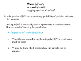
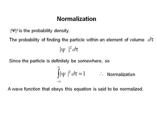
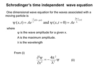
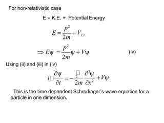
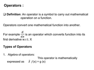
Failure Of Classical Mechanics
Classical mechanics does not provide satisfactory
explanation for phenomena.
1. Black body radiation
2. Photoelectric effect
3. Atomic and molecular spectra
4. Heat capacities of solids
Thus new mechanics was needed to explain the
behaviours of micro particle.
This lead to development of new mechanics known as
“ Quantum mechanics ”
Theory of Wave function
Definition :-
The variable quantity, varying in space & time,
characterizing de-Broglie waves is called the wave function, written as
“Ψ”
 It is desirable to relate the value of wave function associated with a moving
particle at a point at a particular time to the likelihood of finding the particle
of that point at that time.
 Ψ(x, y, z, t) should be such that its magnitude is large in regions where the
probability of finding the particle around a particular position.
 Ψ can be +ve, -ve, real or complex where as the probability is always real
and positive.
Where ||2
*
 AiB*AiB
||2
*A2
i2
B2
A2
B2
 A large value of Ψ 2 means the strong probability of particle’s existance
& vice-versa.
As long as Ψ 2 is not actually zero at a point there is a definite chances.
However small of detecting the particle there.
 Properties of wave function:-
i. Ψmust be normalizable i.e, the integral of Ψ 2 overall space
must be finite.
ii. Ψ must be finite of all points where the particle can be
present.
iii. Because the probability of locating the particle at a point at a
given instant can have only one value, Ψ must be single valued
everywhere in its permissible range.
iv. Ψmust be continuous in all regions of its existance.
v. Partial derivatives of Ψ, i.e.
𝜕Ψ
𝜕𝑥
,
Schrodinger’s time independent wave equation
One dimensional wave equation for the waves associated with a
moving particle is
2
ψ is the wave amplitude for a given x.
A is the maximum amplitude.
λ is the wavelength
From (i)
2

 
4 2

x2
(ii)
2 i
(x)i
(Et px)
(x,t)  Ae and (x,t  0)  Ae 
where
h
mov
 
2
 o

1 m v2
2
h2
2
2
1
h2
m v2m o 

o

  
(iii)
1

2mo K
2
h2
where K is the K.E. for the non-relativistic case
Suppose E is the total energy of the particle
and V is the potential energy of the particle
1

2mo
(E V )
2
h2
This is the time independent (steady state) Schrodinger’s wave
equation for a particle of mass mo, total energy E, potential
energy V, moving along the x-axis.
If the particle is moving in 3-dimensional space then
Equation (ii) now becomes
h2
2mo (E V)
2

 
42
x2
2
 2m
x2
 o
(E V )  0
2
2
 2
 2
 2m
x2
y2
z2
  o
(E V )  0
2
For a free particle V = 0, so the Schrodinger equation for a
free particle
2
 
2mo
E  0
2
2
 
2mo
(E V )  02
This is the time independent (steady state) Schrodinger’s wave
equation for a particle in 3-dimensional space.
i
(Et px)
  Ae
Schrodinger’s time dependent wave equation
Wave equation for a free particle moving in +x direction is
(iii)
p2
x2
2

where E is the total energy and p is the momentum of the particle
Differentiating (i) twice w.r.t. x
(i)
2
x2
2 2
    p 

2
(ii)
Differentiating (i) w.r.t. t

 
iE

t t
 E  i

(iv)
V
 2
2
i
t
 
2m x2
 E    V
Using (ii) and (iii) in (iv)
2m
For non-relativistic case
E = K.E. + Potential Energy
p2
E 
2m
 Vx,t
p2
This is the time dependent Schrodinger’s wave equation for a
particle in one dimension.
Operators :
 Definition: An operator is a symbol to carry out mathematical
operation on a function.
Operators convert one mathematical function into another.
For example
𝑑
𝑑𝑥
is an operator which converts function into its
first derivative w.r.t. X
Types of Operators
1. Algebra of operators:
This operator is mathematically
expressed as 𝐴 𝑓(x) = g (x)
For ex. Let 𝐴 =
𝑑
𝑑𝑥
and f(x) = ax2
𝐴 𝑓(x) =
𝑑
𝑑𝑥
ax2
= 2ax→ ∴ g (x) = 2ax
2.Addition and Substraction operators:
if 𝐴 and 𝐵 are two different operators and f(x) is operand
Then, ( 𝐴 ± 𝐵) f(x) = 𝐴f(x) ± 𝐵f(x)
Ex. Let 𝐴= lo𝑔10 and 𝐵 = f(x) = x
( 𝐴 ± 𝐵) f(x) = (lo𝑔10 ± ) x
= lo𝑔10 x±
𝑥2
2
Commulative and Non – commulative operators : When a
Series of operations are performed on a function sucessively , the result
depends on the sequence in which the operations are performed.
If 𝐴 𝐵 f(x) = 𝐵 𝐴 f(x)
Then two operators 𝐴 and 𝐵 are said to be commutative.
If 𝐴 𝐵 f(x) = 𝐵 𝐴 f(x)
Then two operators 𝐴 and 𝐵 are said to be non- commutative.
Eigen values and Eigen function
Statement: When the result of operating on some function f(x)
gives same function multiplied by a constant (a)
Then function f(x) is called as eigen function and the constant (a)
is called the eigen function
  a 
^
then ^
^
ψ is the eigen function of 
a is the eigen value of 
Q. Suppose is eigen function of operator then find
the eigen value.
Solution.
2x
  e
dx2
d2
^ d2
G 
^
dx2
d2

dx2
G  2x
dx2
d2
 (e )
^
^
G  4e2x
G  4
The eigen value is 4.
Quantum mechanics

Quantum mechanics

  • 2.
    Failure Of ClassicalMechanics Classical mechanics does not provide satisfactory explanation for phenomena. 1. Black body radiation 2. Photoelectric effect 3. Atomic and molecular spectra 4. Heat capacities of solids
  • 3.
    Thus new mechanicswas needed to explain the behaviours of micro particle. This lead to development of new mechanics known as “ Quantum mechanics ”
  • 4.
    Theory of Wavefunction Definition :- The variable quantity, varying in space & time, characterizing de-Broglie waves is called the wave function, written as “Ψ”  It is desirable to relate the value of wave function associated with a moving particle at a point at a particular time to the likelihood of finding the particle of that point at that time.  Ψ(x, y, z, t) should be such that its magnitude is large in regions where the probability of finding the particle around a particular position.  Ψ can be +ve, -ve, real or complex where as the probability is always real and positive.
  • 5.
    Where ||2 *  AiB*AiB ||2 *A2 i2 B2 A2 B2 A large value of Ψ 2 means the strong probability of particle’s existance & vice-versa. As long as Ψ 2 is not actually zero at a point there is a definite chances. However small of detecting the particle there.  Properties of wave function:- i. Ψmust be normalizable i.e, the integral of Ψ 2 overall space must be finite. ii. Ψ must be finite of all points where the particle can be present.
  • 6.
    iii. Because theprobability of locating the particle at a point at a given instant can have only one value, Ψ must be single valued everywhere in its permissible range. iv. Ψmust be continuous in all regions of its existance. v. Partial derivatives of Ψ, i.e. 𝜕Ψ 𝜕𝑥 ,
  • 8.
    Schrodinger’s time independentwave equation One dimensional wave equation for the waves associated with a moving particle is 2 ψ is the wave amplitude for a given x. A is the maximum amplitude. λ is the wavelength From (i) 2    4 2  x2 (ii) 2 i (x)i (Et px) (x,t)  Ae and (x,t  0)  Ae  where
  • 9.
    h mov   2  o  1m v2 2 h2 2 2 1 h2 m v2m o   o     (iii) 1  2mo K 2 h2 where K is the K.E. for the non-relativistic case Suppose E is the total energy of the particle and V is the potential energy of the particle 1  2mo (E V ) 2 h2
  • 10.
    This is thetime independent (steady state) Schrodinger’s wave equation for a particle of mass mo, total energy E, potential energy V, moving along the x-axis. If the particle is moving in 3-dimensional space then Equation (ii) now becomes h2 2mo (E V) 2    42 x2 2  2m x2  o (E V )  0 2 2  2  2  2m x2 y2 z2   o (E V )  0 2
  • 11.
    For a freeparticle V = 0, so the Schrodinger equation for a free particle 2   2mo E  0 2 2   2mo (E V )  02 This is the time independent (steady state) Schrodinger’s wave equation for a particle in 3-dimensional space.
  • 12.
    i (Et px)  Ae Schrodinger’s time dependent wave equation Wave equation for a free particle moving in +x direction is (iii) p2 x2 2  where E is the total energy and p is the momentum of the particle Differentiating (i) twice w.r.t. x (i) 2 x2 2 2     p   2 (ii) Differentiating (i) w.r.t. t    iE  t t  E  i 
  • 13.
    (iv) V  2 2 i t   2mx2  E    V Using (ii) and (iii) in (iv) 2m For non-relativistic case E = K.E. + Potential Energy p2 E  2m  Vx,t p2 This is the time dependent Schrodinger’s wave equation for a particle in one dimension.
  • 14.
    Operators :  Definition:An operator is a symbol to carry out mathematical operation on a function. Operators convert one mathematical function into another. For example 𝑑 𝑑𝑥 is an operator which converts function into its first derivative w.r.t. X Types of Operators 1. Algebra of operators: This operator is mathematically expressed as 𝐴 𝑓(x) = g (x)
  • 15.
    For ex. Let𝐴 = 𝑑 𝑑𝑥 and f(x) = ax2 𝐴 𝑓(x) = 𝑑 𝑑𝑥 ax2 = 2ax→ ∴ g (x) = 2ax 2.Addition and Substraction operators: if 𝐴 and 𝐵 are two different operators and f(x) is operand Then, ( 𝐴 ± 𝐵) f(x) = 𝐴f(x) ± 𝐵f(x) Ex. Let 𝐴= lo𝑔10 and 𝐵 = f(x) = x ( 𝐴 ± 𝐵) f(x) = (lo𝑔10 ± ) x = lo𝑔10 x± 𝑥2 2
  • 16.
    Commulative and Non– commulative operators : When a Series of operations are performed on a function sucessively , the result depends on the sequence in which the operations are performed. If 𝐴 𝐵 f(x) = 𝐵 𝐴 f(x) Then two operators 𝐴 and 𝐵 are said to be commutative. If 𝐴 𝐵 f(x) = 𝐵 𝐴 f(x) Then two operators 𝐴 and 𝐵 are said to be non- commutative.
  • 17.
    Eigen values andEigen function Statement: When the result of operating on some function f(x) gives same function multiplied by a constant (a) Then function f(x) is called as eigen function and the constant (a) is called the eigen function   a  ^ then ^ ^ ψ is the eigen function of  a is the eigen value of 
  • 18.
    Q. Suppose iseigen function of operator then find the eigen value. Solution. 2x   e dx2 d2 ^ d2 G  ^ dx2 d2  dx2 G  2x dx2 d2  (e ) ^ ^ G  4e2x G  4 The eigen value is 4.

Editor's Notes