2. 8 2 Basic Notions and Examples
We note that if f and g are invertible, then the map h is also invertible and its
inverse is given by
h−1 (x, y) = f −1 (x), g −1 (y) .
Now we consider the case of continuous time.
Definition 2.2 A family of maps ϕt : X → X for t ≥ 0 such that ϕ0 = Id and
ϕt+s = ϕt ◦ ϕs for every t, s ≥ 0
is called a semiflow. A family of maps ϕt : X → X for t ∈ R such that ϕ0 = Id and
ϕt+s = ϕt ◦ ϕs for every t, s ∈ R
is called a flow.
We also say that a family of maps ϕt is a dynamical system with continuous time
or simply a dynamical system if it is a flow or a semiflow. We note that if ϕt is a
flow, then
ϕt ◦ ϕ−t = ϕ−t ◦ ϕt = ϕ0 = Id
and thus, each map ϕt is invertible and its inverse is given by ϕt−1 = ϕ−t .
A simple example of a flow is any movement by translation with constant veloc-
ity.
Example 2.2 Given y ∈ Rn , consider the maps ϕt : Rn → Rn defined by
ϕt (x) = x + ty, t ∈ R, x ∈ Rn .
Clearly, ϕ0 = Id and
ϕt+s (x) = x + (t + s)y
= (x + sy) + ty = (ϕt ◦ ϕs )(x).
In other words, the family of maps ϕt is a flow.
Example 2.3 Given two flows ϕt : X → X and ψt : Y → Y , for t ∈ R, the family of
maps αt : X × Y → X × Y defined for each t ∈ R by
αt (x, y) = ϕt (x), ψt (y)
is also a flow. Moreover,
αt−1 (x, y) = ϕ−t (x), ψ−t (y) .
We emphasize that the expression dynamical system is used to refer both to dy-
namical systems with discrete time and to dynamical systems with continuous time.
3. 2.2 Examples with Discrete Time 9
2.2 Examples with Discrete Time
In this section we describe several examples of dynamical systems with discrete
time.
2.2.1 Rotations of the Circle
We first consider the rotations of the circle. The circle S 1 is defined to be R/Z, that
is, the real line with any two points x, y ∈ R identified if x − y ∈ Z. In other words,
S 1 = R/Z = R/∼,
where ∼ is the equivalence relation on R defined by x ∼ y ⇔ x − y ∈ Z. The cor-
responding equivalence classes, which are the elements of S 1 , can be written in the
form
[x] = x + m : m ∈ Z .
In particular, one can introduce the operations
[x] + [y] = [x + y] and [x] − [y] = [x − y].
One can also identify S 1 with [0, 1]/{0, 1}, where the endpoints of the interval [0, 1]
are identified.
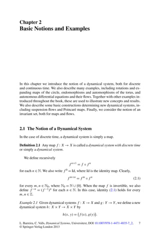
Definition 2.3 Given α ∈ R, we define the rotation Rα : S 1 → S 1 by
Rα [x] = [x + α]
(see Fig. 2.1).
Sometimes, we also write
Rα (x) = x + α mod 1,
thus identifying [x] with its representative in the interval [0, 1). The map Rα could
also be called a translation of the interval. Clearly, Rα : S 1 → S 1 is invertible and
−1
its inverse is given by Rα = R−α .
Now we introduce the notion of a periodic point.
Definition 2.4 Given q ∈ N, a point x ∈ X is said to be a q-periodic point of a map
f : X → X if f q (x) = x. We also say that x ∈ X is a periodic point of f if it is
q-periodic for some q ∈ N.
In particular, the fixed points, that is, the points x ∈ X such that f (x) = x are q-
periodic for any q ∈ N. Moreover, a q-periodic point is kq-periodic for any k ∈ N.
4. 10 2 Basic Notions and Examples
Fig. 2.1 The rotation Rα
Definition 2.5 A periodic point is said to have period q if it is q-periodic but is not
l-periodic for any l < q.
Now we consider the particular case of the rotations Rα of the circle. We verify
that their behavior is very different depending on whether α is rational or irrational.
Proposition 2.1 Given α ∈ R:
1. if α ∈ R Q, then Rα has no periodic points;
2. if α = p/q ∈ Q with p and q coprime, then all points of S 1 are periodic for Rα
and have period q.
Proof We note that [x] ∈ S 1 is q-periodic if and only if [x + qα] = [x], that is, if
and only if qα ∈ Z. The two properties in the proposition follow easily from this
observation.
2.2.2 Expanding Maps of the Circle
In this section we consider another family of maps of S 1 .
5. 2.2 Examples with Discrete Time 11
Fig. 2.2 The expanding
map E2
Definition 2.6 Given an integer m > 1, the expanding map Em : S 1 → S 1 is defined
by
Em (x) = mx mod 1.
For example, for m = 2, we have
2x if x ∈ [0, 1/2),
E2 (x) =
2x − 1 if x ∈ [1/2, 1)
(see Fig. 2.2).
q
Now we determine the periodic points of the expanding map Em . Since Em (x) =
m q x mod 1, a point x ∈ S 1 is q-periodic if and only if
mq x − x = mq − 1 x ∈ Z.
Hence, the q-periodic points of the expanding map Em are
p
x= , for p = 1, 2, . . . , mq − 1. (2.2)
mq−1
Moreover, the number nm (q) of periodic points of Em with period q can be com-
puted easily for each given q (see Table 2.1 for q ≤ 6). For example, if q is prime,
then
nm (q) = mq − m.
6. 12 2 Basic Notions and Examples
Table 2.1 The number
nm (q) of periodic points of q nm (q)
Em with period q
1 m−1
2 m2 − m = m2 − 1 − (m − 1)
3 m3 − m = m3 − 1 − (m − 1)
4 m4 − m2 = m4 − 1 − (m2 − 1)
5 m5 − m = m5 − 1 − (m − 1)
6 m6 − m3 − m2 + m
2.2.3 Endomorphisms of the Torus
In this section we consider a third family of dynamical systems with discrete time.
Given n ∈ N, the n-torus or simply the torus is defined to be
Tn = Rn /Zn = Rn /∼,
where ∼ is the equivalence relation on Rn defined by x ∼ y ⇔ x − y ∈ Zn . The
elements of Tn are thus the equivalence classes
[x] = x + y : y ∈ Zn ,
with x ∈ Rn . Now let A be an n × n matrix with entries in Z.
Definition 2.7 The endomorphism of the torus TA : Tn → Tn is defined by
TA [x] = [Ax] for [x] ∈ Tn .
We also say that TA is the endomorphism of the torus induced by A.
Since A is a linear transformation,
Ax − Ay ∈ Zn when x − y ∈ Zn .
This shows that Ay ∈ [Ax] when y ∈ [x] and hence, TA is well defined.
In general, the map TA may not be invertible, even if the matrix A is invertible.
When TA is invertible, we also say that it is the automorphism of the torus induced
by A. We represent in Fig. 2.3 the automorphism of the torus T2 induced by the
matrix
2 1
A= .
1 1
Now we determine the periodic points of a class of automorphisms of the torus.
Proposition 2.2 Let TA : Tn → Tn be an automorphism of the torus induced by a
matrix A without eigenvalues with modulus 1. Then the periodic points of TA are
the points with rational coordinates, that is, the elements of Qn /Zn .
7. 2.2 Examples with Discrete Time 13
Fig. 2.3 An automorphism of the torus T2
Proof Let [x] = [(x1 , . . . , xn )] ∈ Tn be a periodic point. Then there exist q ∈ N and
y = (y1 , . . . , yn ) ∈ Zn such that Aq x = x + y, that is,
Aq − Id x = y.
Since A has no eigenvalues with modulus 1, the matrix Aq − Id is invertible and one
can write
−1
x = Aq − Id y.
Moreover, since Aq − Id has only integer entries, each entry of (Aq − Id)−1 is a
rational number and thus x ∈ Qn .
Now we assume that [x] = [(x1 , . . . , xn )] ∈ Qn /Zn and we write
p1 pn
(x1 , . . . , xn ) = ,..., , (2.3)
r r
8. 14 2 Basic Notions and Examples
where p1 , . . . , pn ∈ {0, 1, . . . , r − 1}. Since A has only integer entries, for each
q ∈ N we have
p1 p
Aq (x1 , . . . , xn ) = ,..., n + (y1 , . . . , yn )
r r
for some p1 , . . . , pn ∈ {0, 1, . . . , r − 1} and (y1 , . . . , yn ) ∈ Zn . But since the number
of points of the form (2.3) is r n , there exist q1 , q2 ∈ N with q1 = q2 such that
Aq1 (x1 , . . . , xn ) − Aq2 (x1 , . . . , xn ) ∈ Zn .
Assuming, without loss of generality, that q1 > q2 , we obtain
Aq1 −q2 (x1 , . . . , xn ) − (x1 , . . . , xn ) ∈ Zn
q −q2
(see Exercise 2.12) and thus TA1 ([x]) = [x].
The following example shows that Proposition 2.2 cannot be extended to arbi-
trary endomorphisms of the torus.
Example 2.4 Consider the endomorphism of the torus TA : T2 → T2 induced by the
matrix
3 1
A= .
1 1
We note that TA is not an automorphism since det A = 2 (see Exercise 2.12). Now
we observe that
1 1 1 1 1
TA 0, = , , TA , = (0, 0) and TA (0, 0) = (0, 0).
2 2 2 2 2
This shows that the points with rational coordinates (0, 1/2) √ (1/2, 1/2) are not
and √
periodic. On the other hand, the eigenvalues of A are 2 + 2 and 2 − 2, both
without modulus 1.
2.3 Examples with Continuous Time
In this section we give some examples of dynamical systems with continuous time.
2.3.1 Autonomous Differential Equations
We first consider autonomous (ordinary) differential equations, that is, differential
equations not depending explicitly on time. We verify that they give rise naturally
to the concept of a flow.
9. 2.3 Examples with Continuous Time 15
Proposition 2.3 Let f : Rn → Rn be a continuous function such that, given x0 ∈
Rn , the initial value problem
x = f (x),
(2.4)
x(0) = x0
has a unique solution x(t, x0 ) defined for t ∈ R. Then the family of maps ϕt : Rn →
Rn defined for each t ∈ R by
ϕt (x0 ) = x(t, x0 )
is a flow.
Proof Given s ∈ R, consider the function y : R → Rn defined by
y(t) = x(t + s, x0 ).
We have y(0) = x(s, x0 ) and
y (t) = x (t + s, x0 ) = f (x(t + s, x0 )) = f (y(t))
for t ∈ R. In other words, the function y is also a solution of the equation x = f (x).
Since by hypothesis the initial value problem (2.4) has a unique solution, we obtain
y(t) = x t, y(0) = x t, x(s, x0 ) ,
or equivalently,
x(t + s, x0 ) = x t, x(s, x0 ) (2.5)
for t, s ∈ R and x0 ∈ Rn . It follows from (2.5) that ϕt+s = ϕt ◦ ϕs . Moreover,
ϕ0 (x0 ) = x(0, x0 ) = x0 ,
that is, ϕ0 = Id. This shows that the family of maps ϕt is a flow.
Now we consider two specific examples of autonomous differential equations
and we describe the flows that they determine.
Example 2.5 Consider the differential equation
x = −y,
y = x.
If (x, y) = (x(t), y(t)) is a solution, then
x 2 + y 2 = 2xx + 2yy = −2xy + 2yx = 0.
10. 16 2 Basic Notions and Examples
Thus, there exists a constant r ≥ 0 such that
x(t)2 + y(t)2 = r 2 .
Writing
x(t) = r cos θ (t) and y(t) = r sin θ (t),
where θ is some differentiable function, it follows from the identity x = −y that
−rθ (t) sin θ (t) = −r sin θ (t).
Hence, θ (t) = 1 and there exists a constant c ∈ R such that θ (t) = t + c. Thus,
writing
(x0 , y0 ) = (r cos c, r sin c) ∈ R2 ,
we obtain
x(t) r cos(t + c)
=
y(t) r sin(t + c)
cos t · r cos c − sin t · r sin c
=
sin t · r cos c + cos t · r sin c
cos t − sin t x0
= .
sin t cos t y0
Notice that
cos t − sin t
R(t) =
sin t cos t
is a rotation matrix for each t ∈ R. Since R(0) = Id, it follows from Proposition 2.3
that the family of maps ϕt : R2 → R2 defined by
x0 x0
ϕt = R(t)
y0 y0
is a flow. Incidentally, the identity ϕt+s = ϕt ◦ ϕs is equivalent to the identity be-
tween rotation matrices
R(t + s) = R(t)R(s).
Example 2.6 Now we consider the differential equation
x = y,
y = x.
If (x, y) = (x(t), y(t)) is a solution, then
x 2 − y 2 = 2xx − 2yy = 2xy − 2yx = 0.
11. 2.3 Examples with Continuous Time 17
Thus, there exists a constant r ≥ 0 such that
x(t)2 − y(t)2 = r 2 or x(t)2 − y(t)2 = −r 2 . (2.6)
In the first case, one can write
x(t) = r cosh θ (t) and y(t) = r sinh θ (t),
where θ is some differentiable function. Since x = y, we have
rθ (t) sinh θ (t) = r sinh θ (t)
and hence, θ (t) = t + c for some constant c ∈ R. Thus, writing
(x0 , y0 ) = (r cosh c, r sinh c) ∈ R2 ,
we obtain
x(t) r cosh(t + c)
=
y(t) r sinh(t + c)
cosh t · r cosh c + sinh t · r sinh c
=
sinh t · r cosh c + cosh t · sinh c
cosh t sinh t x0 x0
= = S(t) ,
sinh t cosh t y0 y0
where
cosh t sinh t
S(t) = .
sinh t cosh t
In the second case in (2.6), one can write
x(t) = r sinh θ (t) and y(t) = r cosh θ (t).
Proceeding analogously, we find that θ (t) = t + c for some constant c ∈ R. Thus,
writing
(x0 , y0 ) = (r sinh c, r cosh c) ∈ R2 ,
we obtain
x(t) r sinh(t + c)
=
y(t) r cosh(t + c)
sinh t · r cosh c + cosh t · r sinh c
=
cosh t · r cosh c + sinh t · r sinh c
x0
= S(t) .
y0
12. 18 2 Basic Notions and Examples
Notice that S(0) = Id. It follows from Proposition 2.3 that the family of maps
ψt : R2 → R2 defined by
x0 x0
ψt = S(t)
y0 y0
is a flow. In particular, it follows from the identity ψt+s = ψt ◦ ψs that
S(t + s) = S(t)S(s) for t, s ∈ R.
2.3.2 Discrete Time Versus Continuous Time
In this section we describe some relations between dynamical systems with discrete
time and dynamical systems with continuous time.
Example 2.7 Given a flow ϕt : X → X, for each T ∈ R, the map f = ϕT : X → X
is a dynamical system with discrete time. We note that f is invertible and that its
inverse is given by f −1 = ϕ−T . Similarly, given a semiflow ϕt : X → X, for each
T ≥ 0, the map f = ϕT : X → X is a dynamical system with discrete time.
Now we describe a class of semiflows obtained from a dynamical system with
discrete time f : X → X. Given a function τ : X → R+ , consider the set Y obtained
from
Z = (x, t) ∈ X × R : 0 ≤ t ≤ τ (x)
identifying the points (x, τ (x)) and (f (x), 0), for each x ∈ R. More precisely, we
define Y = Z/∼, where ∼ is the equivalence relation on Z defined by
(x, t) ∼ (y, s) ⇔ y = f (x), t = τ (x) and s = 0
(see Fig. 2.4).
Definition 2.8 The suspension semiflow ϕt : Y → Y over f with height τ is defined
for each t ≥ 0 by
ϕt (x, s) = (x, s + t) when s + t ∈ [0, τ (x)] (2.7)
(see Fig. 2.4).
One can easily verify that each suspension semiflow is indeed a semiflow. More-
over, when f is invertible, the family of maps ϕt in (2.7), for t ∈ R, is a flow. It is
called the suspension flow over f with height τ .
Conversely, given a semiflow ϕt : Y → Y , sometimes one can construct a dynam-
ical system with discrete time f : X → X such that the semiflow can be seen as a
suspension semiflow over f .
13. 2.3 Examples with Continuous Time 19
Fig. 2.4 A suspension flow
Fig. 2.5 A Poincaré section
Definition 2.9 A set X ⊂ Y is said to be a Poincaré section for a semiflow ϕt if
τ (x) := inf t > 0 : ϕt (x) ∈ X ∈ R+ (2.8)
for each x ∈ X (see Fig. 2.5), with the convention that inf ∅ = +∞. The number
τ (x) is called the first return time of x to the set X.
Thus, the first return time to X is a function τ : X → R+ . We observe that (2.8)
includes the hypothesis that each point of X returns to X. In fact, each point of X
returns infinitely often to X.
Given a Poincaré section, one can introduce a corresponding Poincaré map.
Definition 2.10 Given a Poincaré section X for a semiflow ϕt , we define its
Poincaré map f : X → X by
f (x) = ϕτ (x) (x).
14. 20 2 Basic Notions and Examples
2.3.3 Differential Equations on the Torus T2
We also consider a class of differential equations on T2 . We recall that two vectors
x, y ∈ R2 represent the same point of the torus T2 if and only if x − y ∈ Z2 .
Example 2.8 Let f, g : R2 → R be C 1 functions such that
f (x + k, y + l) = f (x, y) and g(x + k, y + l) = g(x, y)
for any x, y ∈ R and k, l ∈ Z. Then the differential equation in the plane R2 given
by
x = f (x, y),
(2.9)
y = g(x, y)
can be seen as a differential equation on T2 . Clearly, Eq. (2.9) has unique solutions
(that are global, that is, they are defined for t ∈ R since the torus is compact). Let
ϕt : T2 → T2 be the corresponding flow (see Proposition 2.3).
Now we assume that f takes only positive values. Then each solution ϕt (0, z) =
(x(t), y(t)) of Eq. (2.9) crosses infinitely often the line segment x = 0, which is
thus a Poincaré section for ϕt (see Definition 2.9). The first intersection (for t > 0)
occurs at the time
Tz = inf t > 0 : x(t) = 1 .
We also consider the map h : S 1 → S 1 defined by
h(z) = y(Tz ) (2.10)
(see Fig. 2.6). One can use the C 1 dependence of the solutions of a differential
equation on the initial conditions to show that h is a diffeomorphism, that is, a
bijective (one-to-one and onto) differentiable map with differentiable inverse (see
Exercise 2.20).
For example, if f = 1 and g = α ∈ R, then
ϕt (0, z) = (t, z + tα) mod 1.
Thus, Tz = 1 for each z ∈ R and
h(z) = z + α mod 1 = Rα (z).
2.4 Invariant Sets
In this section we introduce the notion of an invariant set with respect to a dynamical
system.
15. 2.4 Invariant Sets 21
Fig. 2.6 The Poincaré map
determined by the Poincaré
section x = 0
Definition 2.11 Given a map f : X → X, a set A ⊂ X is said to be:
1. f -invariant if f −1 A = A, where
f −1 A = x ∈ X : f (x) ∈ A ;
2. forward f -invariant if f (A) ⊂ A;
3. backward f -invariant if f −1 A ⊂ A.
Example 2.9 Consider the rotation Rα : S 1 → S 1 . For α ∈ Q, each set
γ (x) = Rα (x) : n ∈ Z
n
is finite and Rα -invariant. More generally, if α ∈ Q, then a nonempty set A ⊂ X is
Rα -invariant if and only if it is a union of sets of the form γ (x) (see the discussion
after Definition 2.12). For example, the set Q/Z is Rα -invariant.
On the other hand, for α ∈ R Q, each set γ (x) is also Rα -invariant, but now
it is infinite. Again, a nonempty set A ⊂ X is Rα -invariant if and only if it is a
union of sets of the form γ (x). One can show that each set γ (x) is dense in S 1 (see
Example 3.2) and thus, the closed Rα -invariant sets are ∅ and S 1 .
Example 2.10 Now we consider the expanding map E4 : S 1 → S 1 , given by
⎧
⎪4x
⎪ if x ∈ [0, 1/4),
⎪
⎨4x − 1 if x ∈ [1/4, 2/4),
E4 (x) =
⎪4x − 2 if x ∈ [2/4, 3/4),
⎪
⎪
⎩
4x − 3 if x ∈ [3/4, 1)
16. 22 2 Basic Notions and Examples
Fig. 2.7 The expanding map
E4
(see Fig. 2.7). For example, the set
−n
A= E4 [0, 1/4] ∪ [2/4, 3/4] (2.11)
n≥0
is forward E4 -invariant. We note that A is a Cantor set, that is, A is a closed set
without isolated points and containing no intervals.
We also introduce the notions of orbit and semiorbit.
Definition 2.12 For a map f : X → X, given a point x ∈ X, the set
+
γ + (x) = γf (x) = f n (x) : n ∈ N0
is called the positive semiorbit of x. Moreover, when f is invertible,
−
γ − (x) = γf (x) = f −n (x) : n ∈ N0
is called the negative semiorbit of x and
γ (x) = γf (x) = f n (x) : n ∈ Z
is called the orbit of x.
We note that when f is invertible, a nonempty set A ⊂ X is f -invariant if and
only if it is a union of orbits. Indeed, A ⊂ X is f -invariant if and only if
x∈A ⇔ x ∈ f −1 A ⇔ f (x) ∈ A.
17. 2.4 Invariant Sets 23
By induction, this is equivalent to
x∈A ⇔ f n (x) : n ∈ Z ⊂ A ⇔ γ (x) ∈ A
since f is invertible. Thus, a nonempty set A ⊂ X is f -invariant if and only if
A= γ (x).
x∈A
Now we introduce the notion of an invariant set with respect to a flow or a semi-
flow.
Definition 2.13 Given a flow Φ = (ϕt )t∈R of X, a set A ⊂ X is said to be
Φ-invariant if
ϕt−1 A = A for t ∈ R.
Given a semiflow Φ = (ϕt )t≥0 of X, a set A ⊂ X is said to be Φ-invariant if
ϕt−1 A = A for t ≥ 0.
In the case of flows, since ϕt−1 = ϕ−t for t ∈ R, a set A ⊂ X is Φ-invariant if and
only if
ϕt (A) = A for t ∈ R.
Example 2.11 Consider the differential equation
x = 2y 3 ,
(2.12)
y = −3x.
Each solution (x, y) = (x(t), y(t)) satisfies
3x 2 + y 4 = 6xx + 4y 3 y
= 12xy 3 − 12y 3 x = 0.
Thus, for each set I ⊂ R+ , the union
A= (x, y) ∈ R2 : 3x 2 + y 4 = a
a∈I
is invariant with respect to the flow determined by Eq. (2.12).
We also introduce the notions of orbit and semiorbit for a semiflow.
Definition 2.14 For a semiflow Φ = (ϕt )t≥0 of X, given a point x ∈ X, the set
+
γ + (x) = γΦ (x) = ϕt (x) : t ≥ 0
18. 24 2 Basic Notions and Examples
is called the positive semiorbit of x. Moreover, for a flow Φ = (ϕt )t∈R of X,
−
γ − (x) = γΦ (x) = ϕ−t (x) : t ≥ 0
is called the negative semiorbit of x and
γ (x) = γΦ (x) = ϕt (x) : t ∈ R
is called the orbit of x.
2.5 Exercises
Exercise 2.1 Determine whether the map f : R → R given by f (x) = 3x − 3x 2
has periodic points with period 2.
Exercise 2.2 Determine whether the map f : R → R given by f (x) = x 2 + 1 has
periodic points with period 5.
Exercise 2.3 Given a continuous function f : R → R, show that:
1. if [a, b] ⊂ f ([a, b]), then f has a fixed point in [a, b];
2. if [a, b] ⊃ f ([a, b]), then f has a fixed point in [a, b].
Exercise 2.4 Let f : R → R be a continuous function and let [a, b] and [c, d] be
intervals in R such that
[c, d] ⊂ f [a, b] , [a, b] ⊂ f [c, d] and [a, b] ∩ [c, d] = ∅.
Show that f has a periodic point with period 2.
Exercise 2.5 Show that if f : [a, b] → [a, b] is a homeomorphism (that is, a con-
tinuous bijective function with continuous inverse), then f has no periodic points
with period 3 or larger.
Exercise 2.6 Determine whether there exists a homeomorphism f : R → R with:
1. a periodic point with period 2;
2. a periodic point with period 3.
Exercise 2.7 Show that any power of an expanding map is still an expanding map.
Exercise 2.8 Show that the set of periodic points of the expanding map Em is dense
in S 1 .
19. 2.5 Exercises 25
Exercise 2.9 For each q ∈ N, find the number of q-periodic points of the map
f : R → R defined by f (z) = z2 in the set
R = z ∈ C : |z| = 1 .
Exercise 2.10 Show that the number of periodic points of the expanding map Em
with period p = q r , for q prime and r ∈ N, is given by
nm (p) = mp − mp/q .
Exercise 2.11 Find the smallest E3 -invariant set containing [0, 1/3] ∪ [2/3, 1].
Exercise 2.12 Show that the following properties are equivalent:
1. the endomorphism of the torus TA : Tn → Tn is invertible;
2. x ∈ Zn if and only if Ax ∈ Zn ;
3. |det A| = 1.
Exercise 2.13 Let TA : Tn → Tn be an endomorphism of the torus. Show that for
each x ∈ Qn /Zn , there exists an m ∈ N such that TA (x) is a periodic point of TA .
m
Exercise 2.14 Show that the complement of a forward f -invariant set is backward
f -invariant.
Exercise 2.15 Given a map f : X → X, show that:
1. a set A ⊂ X is f -invariant if and only if f −1 A ⊂ A and f (A) ⊂ A;
2. a set A ⊂ X is f -invariant if and only if X A is f -invariant.
Exercise 2.16 Show that if X is a Poincaré section for a semiflow ϕt , then:
1. ϕt has no fixed points in X;
2. f is invertible when ϕt is a flow.
Exercise 2.17 Find the flow determined by the equation x + 4x = 0.
Exercise 2.18 Find the flow determined by the equation x − 5x + 6x = 0.
Exercise 2.19 Show that the equation x = x 2 does not determine a flow.
Exercise 2.20 Use the C 1 dependence of the solutions of a differential equation on
the initial conditions1 together with the implicit function theorem to show that the
map h defined by (2.10) is a diffeomorphism.
1 Theorem (See for example [12]) If f : D → Rn is a C 1 function in an open set D ⊂ Rn and
ϕ(·, x0 ) is the solution of the initial value problem (2.4), then the function (t, x) → ϕ(t, x) is of
class C 1 .