Downloaded 53 times

![4
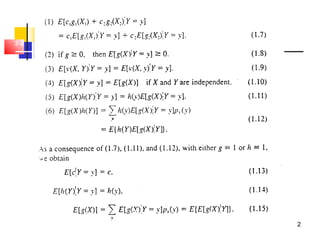
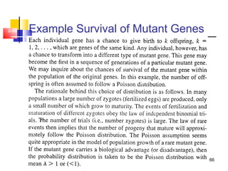
2-4 Discrete-Time Markov Chain
Discrete-time stochastic process {Xn: n = 0,1,2,…}
Takes values in {0,1,2,…}
Memoryless property:
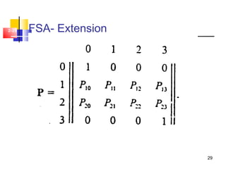
Transition probabilities Pij
Transition probability matrix P=[Pij]
1 1 1 0 0 1
1
{ | , ,..., } { | }
{ | }
n n n n n n
ij n n
P X j X i X i X i P X j X i
P P X j X i
+ − − +
+
= = = = = = =
= = =
0
0, 1ij ij
j
P P
∞
=
≥ =∑](https://image.slidesharecdn.com/2discretemarkovchain-140526230505-phpapp02/85/2-discrete-markov-chain-4-320.jpg)
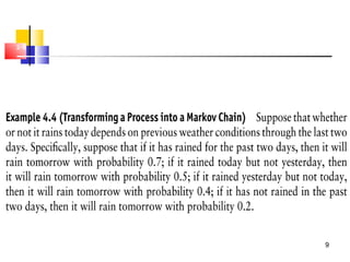
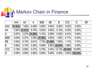

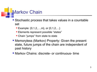
This document discusses Markov chains and related topics: - It defines Markov chains as stochastic processes that take values in a countable set, with the memoryless property that future states only depend on the present state. - It distinguishes between discrete-time and continuous-time Markov chains, and introduces transition probabilities and matrices. - It covers Chapman-Kolmogorov equations for calculating multi-step transition probabilities recursively, and the concept of a stationary distribution when state probabilities converge over time. - Examples discussed include transforming processes into Markov chains, a camera inventory model, and using Markov chains to model bond credit ratings. - Special cases like two-state chains, independent random variables, random walks


![UNIT 1 Machine Learning [KCS-055] (1).pptx](https://cdn.slidesharecdn.com/ss_thumbnails/unit1machinelearningkcs-0551-230208173320-a2f4e13a-thumbnail.jpg?width=640&height=640&fit=bounds)