The document discusses the ladder operator technique for solving the Schrödinger equation for a particle in simple harmonic motion in one dimension. It introduces the Hamiltonian of the system, describes the factorization of the Hamiltonian using raising and lowering operators, and outlines their properties, including commutation relations and their roles as eigenfunction generators. The document aims to detail the process of finding wavefunctions for energy eigenstates and specifically addresses finding the ground state.

1. Ladder operator technique for solving Schr¨odinger
equation for a particle exhibiting simple harmonic
motion in one-dimension1
1 Simple harmonic motion in 1D
For a particle exhibiting simple harmonic motion, Hooke’s law is applicable,
which is given as
F = −k(x − xeq), (1)
where F is the force acting on the particle, k is called force constant, x is
the displacement of the particle from the equilibrium position (xeq). The
negative sign represents that the direction of force on the particle works
in the direction opposite to the displacement. Considering the equilibrium
position at the origin of the Co-ordinate system, Eq. 1 becomes
F = −kx (2)
The force constant k is related to the mass (m) of the particle and angular
velocity of oscillation (ω) by the following relation
k = mω2
(3)
The Hamiltonian for this system is given by
ˆH =
ˆp2
x
2m
+ ˆV (x), (4)
where ˆpx = −i ∂
∂x
, is the linear momentum operator and ˆV (x) is the potential
energy operator for the system. ˆV (x) can be obtained from the definition of
force i.e.
F = −
dV
dx
=⇒ dV = − Fdx
V = k xdx =
1
2
kx2
+ C,
(5)
where C is the constant of integration. Since, at x = 0 (i.e. at equilibrium
position), the total energy of the particle is kinetic in nature. The potential
1
This notes is highly based on the derivations given in the book “Quantum Mechanics”
by David Griffiths. However, you’ll find the derivations and descriptions given in this
notes more detailed.
1

2. energy is zero i.e. V = 0. This means C = 0. Thus,
V =
1
2
kˆx2
=
1
2
mω2
ˆx2
(6)
Using Eq. 6 in Eq. 4, we get
ˆH =
ˆp2
x
2m
+
1
2
mω2
ˆx2
=
1
2m
ˆp2
x + m2
ω2
ˆx2
(7)
Therefore, the Schr¨odinger equation for the particle exhibiting simple har-
monic motion in one-dimension becomes
1
2m
ˆp2
x + m2
ω2
ˆx2
ψ(x) = Eψ(x) (8)
ψ(x) is the eigenstate and E is the eigenvalue of ˆH. Our target is to solve
Eq. 8. This looks a simple second order differential equation. However, be-
cause of the presence of x2
term, it is not really trivial to solve it.
In this notes, we are going to explore the ladder operator technique for
solving Eq. 8.
1.1 Factorization of the Hamiltonian
In ladder operator technique, our first aim will be to factorize the Hamil-
tonian of the system i.e. to express ˆH in Eq. 7 as a product of two or
more operators. If px and x were simple numbers then the task of factor-
ization would be very easy. For example, we could write px + m2
ω2
x2
=
(ipx + mωx) (−ipx + mωx). But, since ˆx and ˆpx are operators and these do
not commute with each other, we can not really get perfect factorization like
this. In spite of this fact, let us try this kind of factorization. We assume
two operators2
,
a+ =
1
√
2 mω
(−iˆpx + mωˆx)
a− =
1
√
2 mω
(iˆpx + mωˆx)
(9)
In short, we can write a± = 1√
2 mω
( iˆpx + mωˆx). Now, with these two new
operators, we can write
a±a =
1
2 mω
( iˆpx + mωˆx) (±iˆpx + mωˆx)
2
Later on, we’ll see why these operators are called ladder operators.
2

3. =
1
2 mω
ˆp2
x iˆpxmωˆx ± imωˆxˆpx + m2
ω2
ˆx2
=
1
2 mω
ˆp2
x + m2
ω2
ˆx2
± imω (ˆxˆpx − ˆpx ˆx) (10)
Since (ˆxˆpx − ˆpx ˆx) represents the commutator [ˆx, ˆpx] and it’s value is i , we
can write
a±a =
1
2 mω
ˆp2
x + m2
ω2
ˆx2
mω
=
1
ω
ˆH
1
2
=⇒ ˆH = ω a±a ±
1
2
(11)
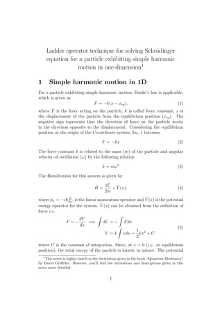
Thus, we see that complete factorization of the Hamiltonian cann not achieved
by using the a+ and a− operators. However, it’s not a big issue. we can sur-
vive with this partial factorization. However, before we proceed, let us first
study some of the important properties of a+ and a− operators, which will
be used in our discussion.
1.2 Some properties of a+ and a− operators
Property 1: Commutation relation between a+ and a−
Let us first find out the commutation relation between a+, a− and ˆH.
[a+, a−] = a+a− − a−a+
=
1
ω
ˆH −
1
2
−
1
ω
ˆH +
1
2
(using Eq. 11)
=⇒ [a+, a−] = 1
(12)
Thus, a+ and a− operators do not commute with each other.
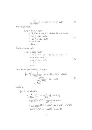
Property 2: Commutation relation between a± and ˆH
a+, ˆH =a+
ˆH − ˆHa+
=
1
√
2 mω
(−iˆpx + mωˆx)
1
2m
ˆp2
x + m2
ω2
ˆx2
−
1
2m
ˆp2
x + m2
ω2
ˆx2 1
√
2 mω
(−iˆpx + mωˆx)
=
1
2m
√
2 mω
−iˆp3
x + mωˆxˆp2
x − im2
ω2
ˆpx ˆx2
+ m3
ω3
ˆx3
− −iˆp3
x − im2
ω2
ˆx2
ˆpx + mωˆp2
x ˆx + m3
ω3
ˆx3
3

4. =
1
2m
√
2 mω
mω ˆx, ˆp2
x + im2
ω2
ˆx2
, ˆpx (13)
Now, we can write
ˆx, ˆp2
x = ˆxˆpx ˆpx − ˆpx ˆpx ˆx
= (i + ˆpx ˆx) ˆpx − ˆpx ˆpx ˆx (Using ˆxˆpx − ˆpx ˆx = i )
= i ˆpx + ˆpx ˆxˆpx − ˆpx ˆpx ˆx
= i ˆpx + ˆpx (ˆxˆpx − ˆpx ˆx)
= i ˆpx + ˆpxi
= 2i ˆpx
(14)
Similarly, we can write
ˆx2
, ˆpx = ˆxˆxˆpx − ˆpx ˆxˆx
= ˆx (i + ˆpx ˆx) − ˆpx ˆxˆx (Using ˆxˆpx − ˆpx ˆx = i )
= i ˆx + ˆxˆpx ˆx − ˆpx ˆxˆx
= i ˆx + (ˆxˆpx − ˆpx ˆx) ˆx
= i ˆx + i ˆx
= 2i ˆx
(15)
Using Eq. 14 and 15 in Eq. 13, we get
a+, ˆH =
1
2m
√
2 mω
mω × 2i ˆpx + im2
ω2
× 2i ˆx
= −
2 mω
2m
√
2 mω
(−iˆpx + mωˆx)
= − ωa+
(16)
Similarly,
a−, ˆH =a−
ˆH − ˆHa−
=
1
√
2 mω
(iˆpx + mωˆx)
1
2m
ˆp2
x + m2
ω2
ˆx2
−
1
2m
ˆp2
x + m2
ω2
ˆx2 1
√
2 mω
(iˆpx + mωˆx)
=
1
2m
√
2 mω
iˆp3
x + mωˆxˆp2
x + im2
ω2
ˆpx ˆx2
+ m3
ω3
ˆx3
− iˆp3
x + im2
ω2
ˆx2
ˆpx + mωˆp2
x ˆx + m3
ω3
ˆx3
4

5. =
1
2m
√
2 mω
mω ˆx, ˆp2
x − im2
ω2
ˆx2
, ˆpx
=
1
2m
√
2 mω
mω × 2i ˆpx − im2
ω2
× 2i ˆx
=
2 mω
2m
√
2 mω
{iˆpx + mωˆx} = ωa−
Thus,
a±, ˆH = ωa± (17)
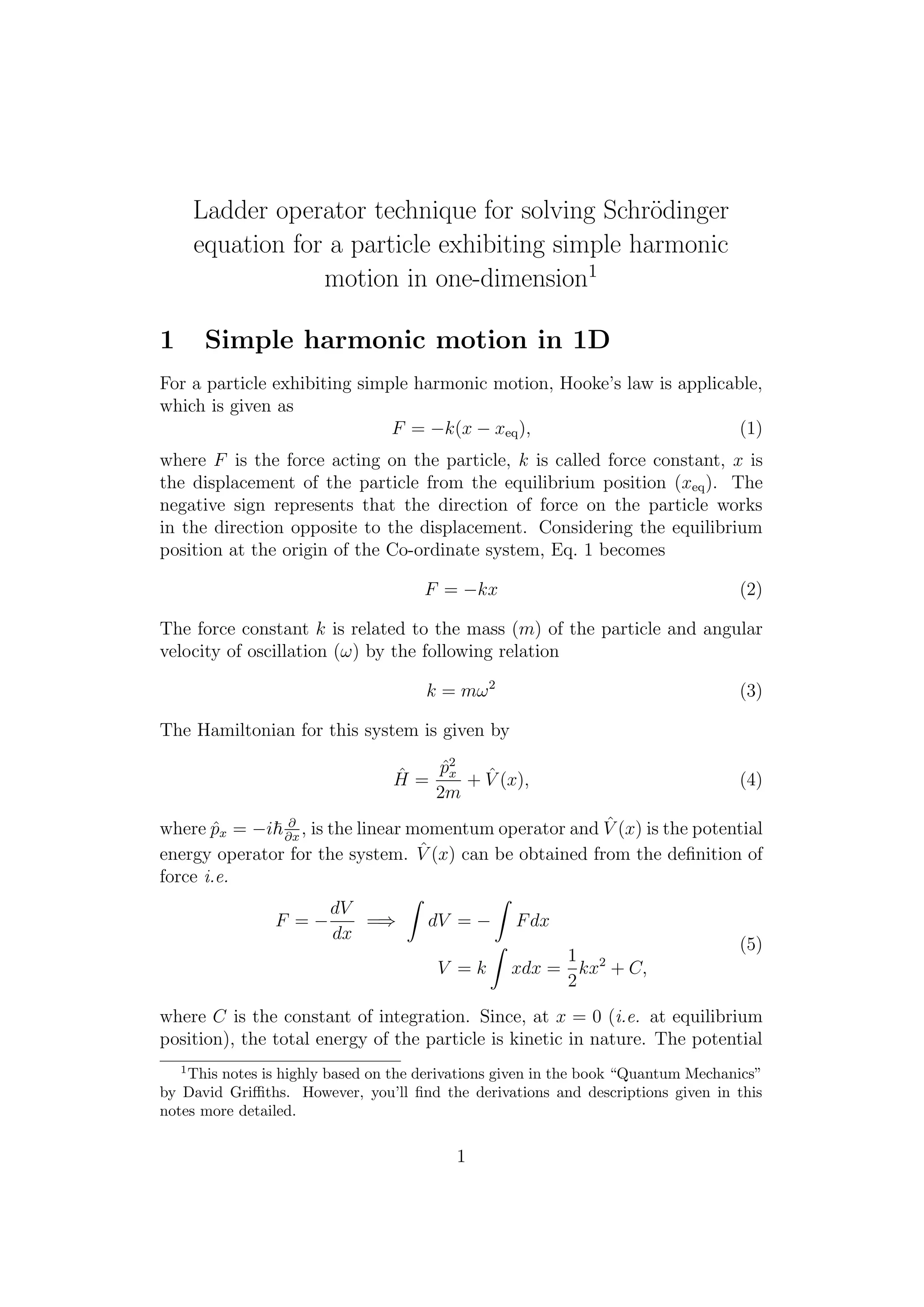
Property 3: a+ and a− behave as raising and lowering operators
respectively
First lets prove that a+ acts as a raising operator. Let ψ(x) be an eigenfunc-
tion of the Hamiltonian ˆH and E be the corresponding eigenvalue.
ˆHψ(x) = Eψ(x) (18)
To prove that a+ is a raising operator, we need to show that when it operates
over some eigenfunction of ˆH then it yields the next higher eigenfunction of
ˆH. Thus, we consider a+ψ(x) and check whether this is the next higher
eigenfunction of ˆH or not.
ˆHa+ψ(x) = ω a+a− +
1
2
a+ψ(x) (Using Eq. 11)
= ω a+a−a+ +
1
2
a+ ψ(x)
= ωa+ a−a+ +
1
2
ψ(x)
= a+ ω 1 + a+a− +
1
2
ψ(x) (Using Eq. 12)
= a+ ω a+a− +
1
2
ψ(x) + ωψ(x)
= a+
ˆHψ(x) + ωψ(x) (Using Eq. 11)
= a+ [Eψ(x) + ωψ(x)]
ˆHa+ψ(x) = (E + ω) a+ψ(x) (19)
Thus, if ψ(x) be an eigenfunction of ˆH with eigenvalue E, then a+ψ(x) will
also be an eigenfunction of ˆH with eigenvalue (E + ω). Therefore, a+ when
operates on an eigenfunction of ˆH, it generates another eigenfunction of ˆH,
with eigenvalue (E + ω), which proves that a+ is a raising operator. If we
5

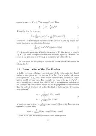
6. apply a+ once again i.e. a2
+ψ(x) then this will generate the second higher
eigenfunction with eigenvalues (E + 2 ω).
Now, to prove that a− is a lowering operator, we need to show that
when it operates over some eigenfunction of ˆH then it yields the next lower
eigenfunction of ˆH. Thus, we consider a−ψ(x) and check whether this is the
next lower eigenfunction of ˆH or not.
ˆHa−ψ(x) = ω a−a+ −
1
2
a−ψ(x) (Using Eq. 11)
= ω a−a+a− −
1
2
a− ψ(x)
= ωa− a+a− −
1
2
ψ(x)
= a− ω a−a+ − 1 −
1
2
ψ(x) (Using Eq. 12)
= a− ω a−a+ −
1
2
ψ(x) − ωψ(x)
= a−
ˆHψ(x) − ωψ(x) (Using Eq. 11)
= a− [Eψ(x) − ωψ(x)]
ˆHa−ψ(x) = (E − ω) a−ψ(x) (20)
Thus, if ψ(x) be an eigenfunction of ˆH with eigenvalue E, then a−ψ(x) will
also be an eigenfunction of ˆH with eigenvalue (E − ω). Therefore, a− when
operates on an eigenfunction of ˆH, it generates another eigenfunction of ˆH,
with eigenvalue (E − ω), which proves that a− is a lowering operator. If
we apply a− once again i.e. a2
−ψ(x) then this will generate the second lower
eigenfunction with eigenvalues (E − 2 ω).
We’ll study some more properties related to our raising and lowering
operators. However, before that we need to find out the ground state (lowest
energy state for our simple harmonic oscillator.
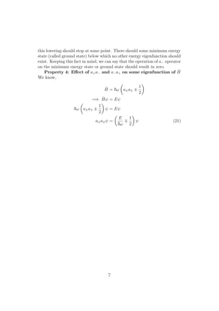
1.3 Finding out the wavefunction of the lowest energ
state of the simple harmonic oscillator
We have seen above that a− behaves as a lowering operator. That means,
if we apply a− operator on some eigenfunction of ˆH then the result will
be another eigenfunction of ˆH with eigenvalue ω less than the previous
eigenfunction. If we keep on applying a− on the eigenfunction then we’ll
keep on getting lower and lower energy eigenfunctions. However, in reality,
6

7. this lowering should stop at some point. There should some minimum energy
state (called ground state) below which no other energy eigenfunction should
exist. Keeping this fact in mind, we can say that the operation of a− operator
on the minimum energy state or ground state should result in zero.
Property 4: Effect of a+a− and a−a+ on some eigenfunction of ˆH
We know,
ˆH = ω a±a ±
1
2
=⇒ ˆHψ = Eψ
ω a±a ±
1
2
ψ = Eψ
a±a ψ =
E
ω
1
2
ψ (21)
7