Continuous random variables and probability distribution

4
Continuous Random
Variables and
Probability Distributions
Stat 4570/5570
Material from Devore’s book (Ed 8) – Chapter 4 - and Cengage

2
Continuous r.v.
A random variable X is continuous if possible values
comprise either a single interval on the number line or a
union of disjoint intervals.
Example: If in the study of the ecology of a lake, X, the r.v.
may be depth measurements at randomly chosen
locations.
Then X is a continuous r.v. The range for X is the minimum
depth possible to the maximum depth possible.

3
Continuous r.v.
In principle variables such as height, weight, and
temperature are continuous, in practice the limitations of
our measuring instruments restrict us to a discrete (though
sometimes very finely subdivided) world.
However, continuous models often approximate real-world
situations very well, and continuous mathematics (calculus)
is frequently easier to work with than mathematics of
discrete variables and distributions.

4
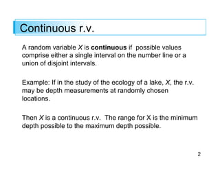
Probability Distributions for Continuous Variables
Suppose the variable X of interest is the depth of a lake at
a randomly chosen point on the surface.
Let M = the maximum depth (in meters), so that any
number in the interval [0, M] is a possible value of X.
If we “discretize” X by measuring depth to the nearest
meter, then possible values are nonnegative integers less
than or equal to M.
The resulting discrete distribution of depth can be pictured
using a probability histogram.

5
If we draw the histogram so that the area of the rectangle
above any possible integer k is the proportion of the lake
whose depth is (to the nearest meter) k, then the total area
of all rectangles is 1:
Probability histogram of depth measured to the nearest meter

6
If depth is measured much more accurately, each rectangle
in the resulting probability histogram is much narrower,
though the total area of all rectangles is still 1.
Probability histogram of depth measured to the nearest centimeter

7
If we continue in this way to measure depth more and more
finely, the resulting sequence of histograms approaches a
smooth curve.
Because for each histogram the total area of all rectangles
equals 1, the total area under the smooth curve is also 1.
A limit of a sequence of discrete histograms

8
Definition
Let X be a continuous r.v. Then a probability distribution
or probability density function (pdf) of X is a function f(x)
such that for any two numbers a and b with a ≤ b, we have
The probability that X is in the interval [a, b] can be
calculated by integrating the pdf of the r.v. X.
P(a  X  b) =
Z b
a
f(x)dx

9
The probability that X takes on a value in the interval [a, b]
is the area above this interval and under the graph of the
density function:
P(a ≤ X ≤ b) = the area under the density curve between a and b

10
For f(x) to be a legitimate pdf, it must satisfy the following
two conditions:
1. f(x) ≥ 0 for all x
2. = area under the entire graph of f(x) = 1

11
Example
Consider the reference line connecting the valve stem on a
tire to the center point.
Let X be the angle measured clockwise to the location of an
imperfection. One possible pdf for X is

12
Example, cont
The pdf is graphed in Figure 4.3.
The pdf and probability from Example 4
Figure 4.3
cont’d

13
Example , cont
Clearly f(x) ≥ 0. How can we show that the area of this pdf
is equal to 1?
How do we calculate P(90 <= X <= 180)?
The probability that the angle of occurrence is within 90° of
the reference line (reference line is at 0 degrees)?
cont’d

14
Because whenever 0 ≤ a ≤ b ≤ 360 in Example 4.4 and
P(a ≤ X ≤ b) depends only on the width b – a of the interval,
X is said to have a uniform distribution.
Definition
A continuous rv X is said to have a uniform distribution
on the interval [A, B] if the pdf of X is

15
Example
“Time headway” in traffic flow is the elapsed time between
the time that one car finishes passing a fixed point and the
instant that the next car begins to pass that point.
Let X = the time headway for two randomly chosen
consecutive cars on a freeway during a period of heavy
flow.
This pdf of X is essentially the one suggested in “The Statistical Properties of
Freeway Traffic” (Transp. Res., vol. 11: 221–228):

16
Example , cont
The graph of f(x) is given in Figure 4.4; there is no density
associated with headway times less than .5, and headway
density decreases rapidly (exponentially fast) as x
increases from .5.
The density curve for time headway in Example 5
Figure 4.4
cont’d

17
Example
Clearly, f(x) ≥ 0; and
What is the probability that headway time is at most 5
seconds?
cont’d
Z 1
1
f(x)dx =
Z 0.5
1
0 dx +
Z 1
0.5
0.15e 0.15(x 0.5)
dx
= 0.15e0.075
Z 1
0.5
e 0.15x
dx = 1

19
The Cumulative Distribution Function
The cumulative distribution function F(x) for a
continuous rv X is defined for every number x by
F(x) = P(X ≤ x) =
For each x, F(x) is the area under the density curve to the
left of x. This is illustrated in Figure 4.5, where F(x)
increases smoothly as x increases.
Figure 4.5
A pdf and associated cdf

20
Example
Let X, the thickness of a certain metal sheet, have a
uniform distribution on [A, B].
The density function is shown in Figure 4.6.
Figure 4.6
The pdf for a uniform distribution

21
Example , cont
For x < A, F(x) = 0, since there is no area under the graph
of the density function to the left of such an x.
For x ≥ B, F(x) = 1, since all the area is accumulated to the
left of such an x. Finally for A ≤ x ≤ B,
cont’d

22
Example , cont
The entire cdf is
The graph of this cdf appears in Figure 4.7.
Figure 4.7
The cdf for a uniform distribution
cont’d

23
Using F(x) to Compute Probabilities

24
Percentiles of a Continuous Distribution
When we say that an individual’s test score was at the 85th
percentile of the population, we mean that 85% of all
population scores were below that score and 15% were
above.
Similarly, the 40th percentile is the score that exceeds 40%
of all scores and is exceeded by 60% of all scores.

25
Proposition
Let p be a number between 0 and 1. The (100p)th
percentile of the distribution of a continuous rv X, denoted
by η(p), is defined by
η(p) is the specific value such that 100p% of the area
under the graph of f(x) lies to the left of η(p) and 100(1 – p)
% lies to the right.
p = F(⌘(p)) =
Z ⌘(p)
1
f(y)dy

26
Thus η(.75), the 75th percentile, is such that the area under
the graph of f(x) to the left of η(.75) is .75.
Figure 4.10 illustrates the definition.
Figure 4.10
The (100p)th percentile of a continuous distribution

27
Example 9
The distribution of the amount of gravel (in tons) sold by a
particular construction supply company in a given week is a
continuous rv X with pdf
What is the cdf of sales for any x? How do you use this to
find the probability that X is less than .25? What about the
probability that X is greater than .75? What about
P(.25 < X < .75)?

28
Example 9
The graphs of both f(x) and F(x) appear in Figure 4.11.
Figure 4.11
The pdf and cdf for Example 4.9
cont’d

29
Example 9
How do we find the 40th percentile of this distribution?
How would you find the median of this distribution?
cont’d

30
Definition
The median of a continuous distribution, denoted by , is
the 50th percentile, so satisfies .5 = F( ) That is, half the
area under the density curve is to the left of and half is to
the right of . The 25th percentile is called the lower
quartile and the 75th percentile is called the upper
quartile.

31
Expected Values
Definition
The expected (or mean) value of a continuous r.v. X with
the pdf f(x) is:
µX = E(X) =
Z 1
1
x · f(x)dx

32
Example, cont
Back to the gravel example, the pdf of the amount of
weekly gravel sales X is:
What is EX?

33
Expected Values of functions of r.v.
If h(X) is a function of X, then
For h(X) = aX + b, a linear function,
µh(X) = E[h(X)] =
Z 1
1
h(x) · f(x) dx
E[h(X)] = E[aX + b] = aE[X] + b

34
Variance
The variance of a continuous random variable X with pdf
f(x) and mean value µ is
The standard deviation (SD) of X is
When h(X) = aX + b,
2
X = V (X) =
Z 1
1
(x µ)2
· f(x) dx
= E[(X E(X))2
]
= E(X2
) E(X)2
X =
p
V (X)
V [h(X)] = V [aX + b] = a2
· 2
X and aX+b = |a| · X

35
Example, cont.
How do we compute the variance for the weekly
gravel sales example?

36
The Normal Distribution
The normal distribution is probably the most important
distribution in all of probability and statistics.
Many populations have distributions that can be fit very
closely by an appropriate normal (or Gaussian, bell) curve.
Examples: height, weight, and other physical
characteristics, scores on various tests, etc.

37
Definition
A continuous r.v. X is said to have a normal distribution
with parameters µ and σ > 0 (or µ and σ 2), if the pdf of X is
• e has approximate value 2.71828
• π has approximate value 3.14159.
f(x; µ, ) =
1
p
2⇡
e (x µ)2
/2 2
where 1 < x < 1

38
The statement that X is normally distributed with
parameters µ and σ2 is often abbreviated X ~ N(µ, σ2).
Clearly f(x; µ, σ) ≥ 0, but a somewhat complicated calculus
argument must be used to verify that f(x; µ, σ) dx = 1.
Similarly, it can be shown that E(X) = µ and V(X) = σ2, so
the parameters are the mean and the standard deviation of
X.

39
Figure below presents graphs of f(x; µ, σ) for several
different (µ, σ) pairs.
Two different normal density curves Visualizing µ and σ for a normal
distribution

40
(z) =
Z z
1
f(y; 0, 1) dy
f(z; 0, 1) =
1
p
2⇡
e z2
/2
where 1 < z < 1
The Standard Normal Distribution
The normal distribution with parameter values µ = 0 and
σ = 1 is called the standard normal distribution.
A r.v. with this distribution is called a standard normal
random variable and is denoted by Z. Its pdf is:
The graph of f(z; 0, 1) is called the standard normal curve.
Its inflection points are at 1 and –1. The cdf of the standard normal is
note we use the special notation Φ(z) for the cdf of Z.

41
• The standard normal distribution rarely occurs naturally.
• Instead, it is a reference distribution from which information about
other normal distributions can be obtained via a simple formula.
• These probabilities can then be found “normal tables”.
• This can also be computed with a single command in R.

42
Figure below illustrates the probabilities tabulated in Table
A.3:

43
Example
P(Z ≤ 1.25) = (1.25), a probability that is tabulated in a
normal table.
What is this probability?
Figure below illustrates this probability:
cont’d

44
Example , cont.
b) P(Z ≥ 1.25) = ?
c) Why does P(Z ≤ –1.25) = P(Z >= 1.25)? What is
(–1.25)?
d) How do we calculate P(–.38 ≤ Z ≤ 1.25)?
cont’d

45
Example
The 99th percentile of the standard normal distribution is
that value of z such that the area under the z curve to the
left of the value is .99
Tables give for fixed z the area under the standard normal
curve to the left of z, whereas now –
we have the area and want the value of z.
This is the “inverse” problem to P(Z ≤ z) = ?
How can the table be used for this?

46
Example
By symmetry, the first percentile is as far below 0 as the
99th is above 0, so equals –2.33 (1% lies below the first
and also above the 99th).
cont’d

47
Percentiles of the Standard Normal Distribution
If p does not appear in a table, what can we do?
What is the 95th percentile of the normal distribution?

48
zα Notation
In statistical inference, we need the z values that give
certain tail areas under the standard normal curve.
There, this notation will be standard:
zα will denote the z value for which α of the area under
the z curve lies to the right of zα.

49
zα Notation for z Critical Values
For example, z.10 captures upper-tail area .10, and z.01
captures upper-tail area .01.
Since α of the area under the z curve lies to the right of zα,
1 – α of the area lies to its left.
Thus zα is the 100(1 – α)th percentile of the standard
normal distribution.
Similarly, what does –zα mean?

50
Example – critical values
z.05 is the 100(1 – .05)th = 95th percentile of the standard
normal distribution, so z.05 = 1.645.
The area under the standard normal curve to the left of
–z.05 is also .05

51
Nonstandard Normal Distributions
When X ~ N(µ, σ 2), probabilities involving X are computed
by “standardizing.” The standardized variable is (X – µ)/
σ.
Subtracting µ shifts the mean from µ to zero, and then
dividing by σ scales the variable so that the standard
deviation is 1 rather than σ.
Proposition
If X has a normal distribution with mean µ and standard
deviation σ, then
is distributed standard normal.

52
Why do we standardize normal random variables?
Equality of nonstandard and standard normal curve areas

53
has a standard normal distribution. Thus

54
THE NORMAL
DISTRIBUTION IN R.

56
The Exponential Distributions
The family of exponential distributions provides probability
models that are very widely used in engineering and
science disciplines. Examples?
Definition
X is said to have an exponential distribution with the rate
parameter λ (λ > 0) if the pdf of X is

57
Integration by parts give the following results:
How would we set up the calculation for EX?
Both the mean and standard deviation of the exponential
distribution equal 1/λ.
CDF:

58
Another important application of the exponential distribution
is to model the distribution of lifetimes, or times to an
event.
A partial reason for the popularity of such applications is
the “memoryless” property of the Exponential
distribution.

59
Suppose a light bulb’s lifetime is exponentially distributed
with parameter λ.
Say you turn the light on, and then we leave and come
back after t0 hours to find it still on. What is the probability
that the light bulb will last for at least additional t hours?
In symbols, we are looking for P(X ≥ t + t0 | X ≥ t0).
How would we calculate this?

60
The Chi-Squared Distribution
Definition
Let v be a positive integer. Then a random variable X is
said to have a chi-squared distribution with parameter v if
the pdf of X is the gamma density with α = v/2 and β = 2.
The pdf of a chi-squared rv is thus
The parameter is called the number of degrees of
freedom (df) of X. The symbol χ2 is often used in place of
“chi-squared.”
(4.10)

61
The Weibull Distribution
The Weibull distribution is used similarly to the exponential
distribution to model times to an event, but with an extra
parameter included for flexilibility.
Definition
A random variable X is said to have a Weibull distribution
with parameters α and β (α > 0, β > 0) if the pdf of X is
What is this distribution if alpha = 1?
(4.11)

62
Both α and β can be varied to obtain a number of different-
looking density curves, as illustrated below.
Weibull density curves

63
β is called a scale parameter, since different values stretch
or compress the graph in the x direction, and α is
referred to as a shape parameter.
β Integrating to obtain E(X) and E(X2) yields
The computation of µ and σ2 requires use of the gamma
function.

64
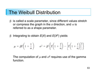
The Beta Distribution
So far, all families of continuous distributions (except for the
uniform distribution) had positive density over an infinite
interval.
The beta distribution provides positive density only for X in
an interval of finite length [A,B].
The standard beta distribution is commonly used to model
variation in the proportion or percentage of a quantity
occurring in different samples. Examples?

65
Definition
A random variable X is said to have a beta distribution
with parameters α, β (both positive), A, and B if the pdf of
X is
The case A = 0, B = 1 gives the standard beta
distribution.

66
Figure below illustrates several standard beta pdf’s.
Standard beta density curves

67
Graphs of the general pdf are similar, except they are
shifted and then stretched or compressed to fit over [A, B].
Unless α and β are integers, integration of the pdf to
calculate probabilities is difficult. Either a table of the
incomplete beta function or appropriate software should be
used.
The mean and variance of X are

68
Example 1
Suppose the pdf of the magnitude X of a dynamic load on a
bridge (in newtons) is
What are F(x), E(X), and Var(X)?

69
Example 1
The graphs of f(x) and F(x) are shown in Figure 4.9.
The pdf and cdf for Example 4.7
cont’d

70
Example 1
What is the probability that the load is between 1 and 1.5?
The probability that the load exceeds 1?
The average load? The median load?
cont’d

71
Example 2
The time that it takes a driver to react to the brake lights on
a decelerating vehicle is critical in helping to avoid rear-end
collisions.
The article “Fast-Rise Brake Lamp as a Collision-
Prevention Device” (Ergonomics, 1993: 391–395) suggests
that reaction time for an in-traffic response to a brake signal
from standard brake lights can be modeled with a normal
distribution having mean value 1.25 sec and standard
deviation of .46 sec.
What is the probability that reaction time is between 1.00
sec and 1.75 sec?

Continuous random variables and probability distribution

More Related Content

Similar to Continuous random variables and probability distribution

Recently uploaded

Continuous random variables and probability distribution