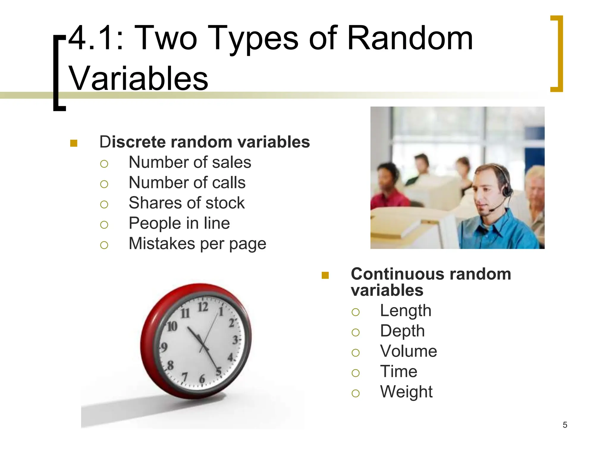
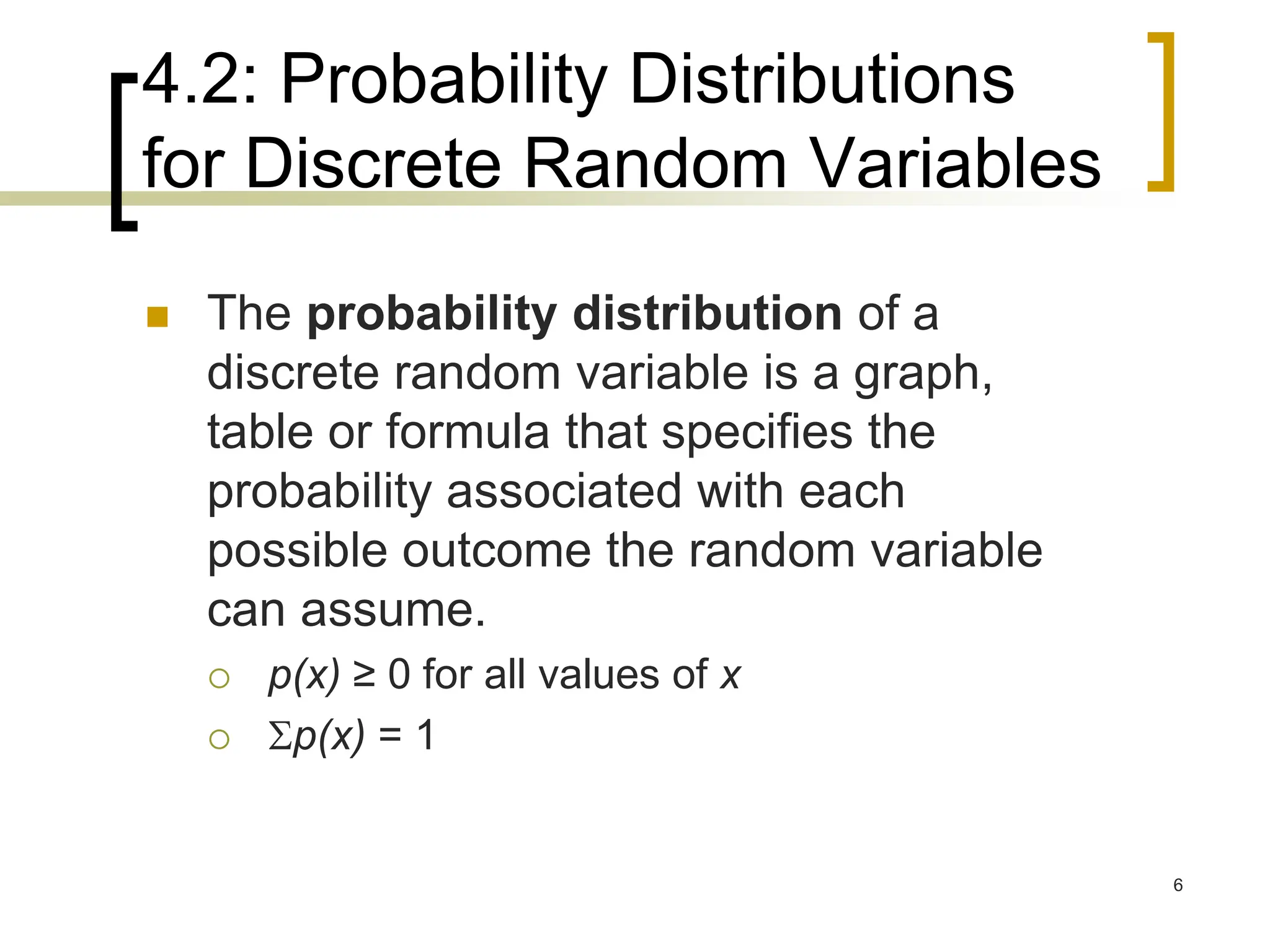
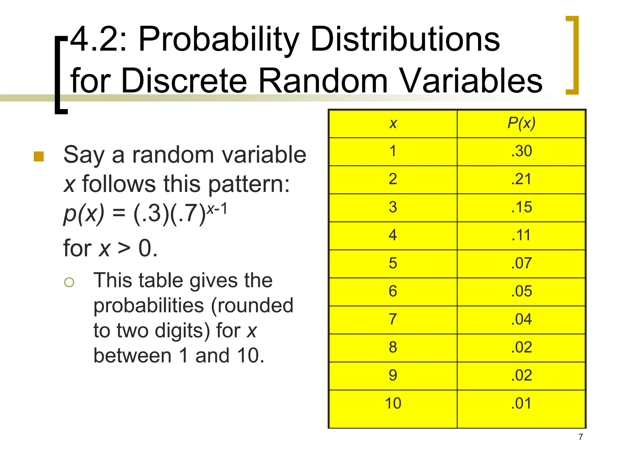
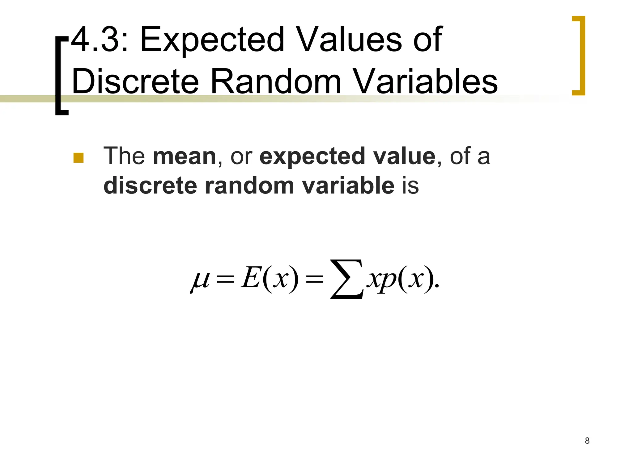
This document discusses probability distributions for discrete random variables. It introduces the concepts of discrete and continuous random variables and gives examples of each. Probability distributions describe the probabilities associated with all possible outcomes of a random variable. The chapter covers the binomial, Poisson, and hypergeometric distributions. It defines key terms like mean, variance, and expected value and provides examples of how to calculate probabilities using these various distributions.
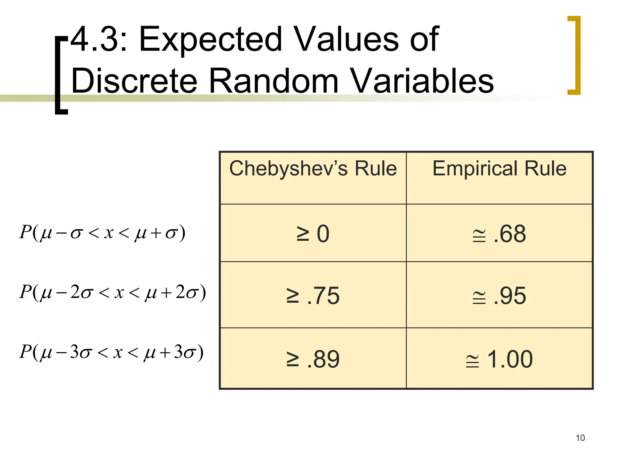
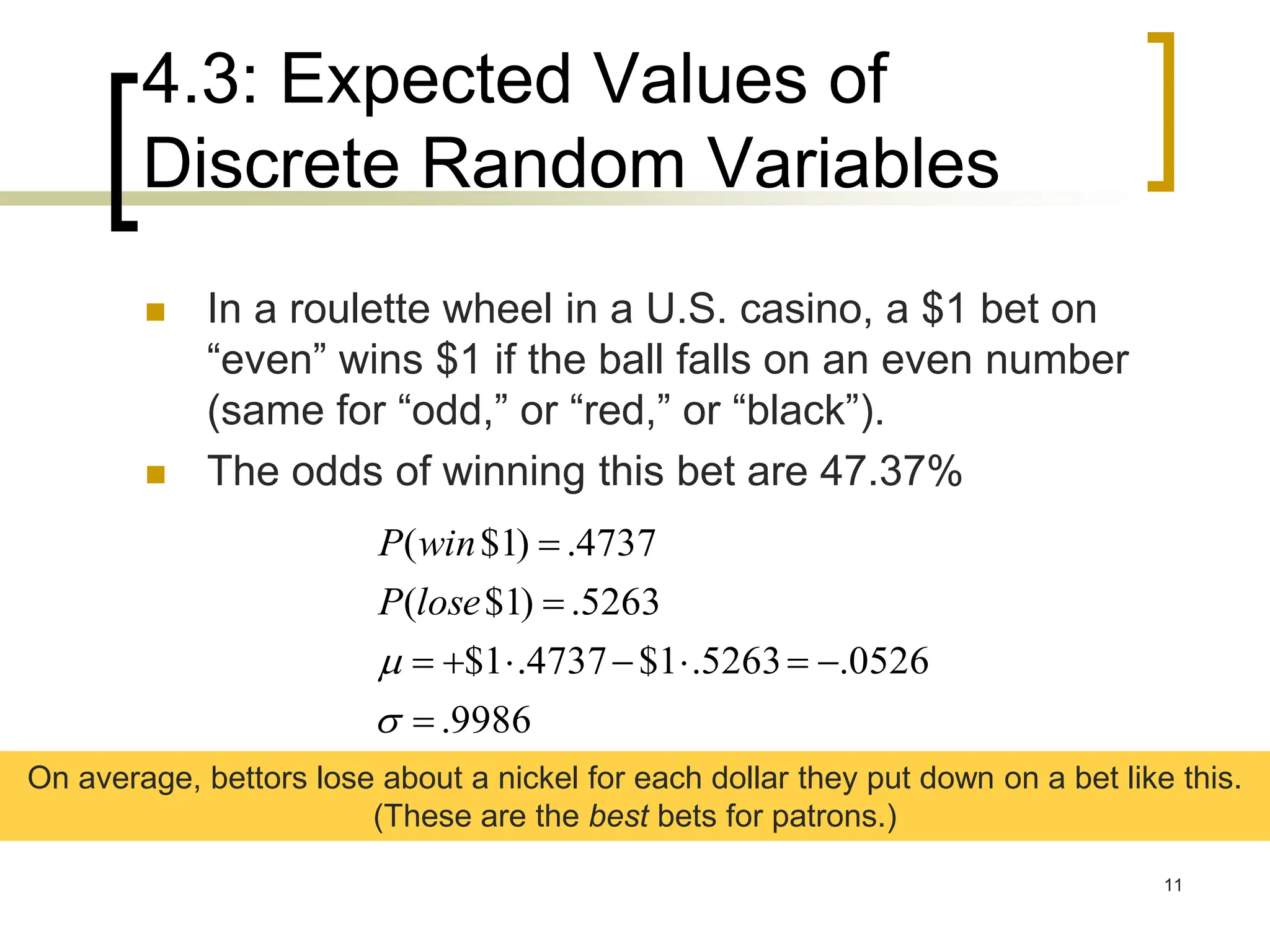
![4.3: Expected Values of
Discrete Random Variables
The variance of a discrete random
variable x is
The standard deviation of a discrete
random variable x is
2 2 2
[( ) ] ( ) ( ).
E x x p x
2 2 2
[( ) ] ( ) ( ).
E x x p x
9](https://image.slidesharecdn.com/group4-randomvariableanddistribution-151014015655-lva1-app6891-240119040056-56ef7b27/75/group4-randomvariableanddistribution-151014015655-lva1-app6891-pdf-9-2048.jpg)


![4.5: The Poisson Distribution
47
Example 1
een on a 1-day safari is 5. What is the probability that tourists will
see fewer than four lions on the next 1-day safari?
Solution: This is a Poisson experiment in
Suppose the average number of lions s which we know the
following:
μ = 5;
x = 0, 1, 2, or 3;
e = 2.71828; since e is a constant equal to approximately
2.71828.
To solve this problem, we need to find the probability that tourists will see
0, 1, 2, or 3 lions. Thus, we need to calculate the sum of four probabilities:
P(0; 5) + P(1; 5) + P(2; 5) + P(3; 5). To compute this sum, we use the Poisson
formula:
P(x < 3, 5) = P(0; 5) + P(1; 5) + P(2; 5) + P(3; 5)
P(x < 3, 5) = [ (e-5)(50) / 0! ] + [ (e-5)(51) / 1! ] + [ (e-5)(52) / 2! ] + [ (e-5)(53) / 3!
]
P(x < 3, 5) = [ (0.006738)(1) / 1 ] + [ (0.006738)(5) / 1 ] + [ (0.006738)(25) / 2
] + [ (0.006738)(125) / 6 ]
P(x < 3, 5) = [ 0.0067 ] + [ 0.03369 ] + [ 0.084224 ] + [ 0.140375 ]
P(x < 3, 5) = 0.2650
Thus, the probability of seeing at no more than 3 lions is 0.2650.](https://image.slidesharecdn.com/group4-randomvariableanddistribution-151014015655-lva1-app6891-240119040056-56ef7b27/75/group4-randomvariableanddistribution-151014015655-lva1-app6891-pdf-47-2048.jpg)