Downloaded 2,201 times


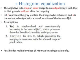
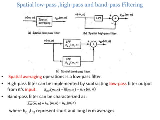
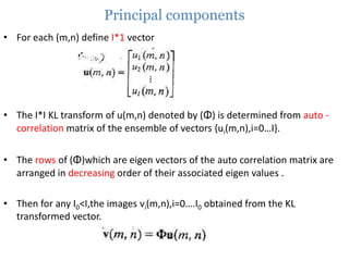
![Spatial-Frequency domain enhancement methods
Spatial domain enhancement methods:
• Spatial domain techniques are performed to the image plane itself and
they are based on direct manipulation of pixels in an image.
• The operation can be formulated as g(x,y) = T[f(x,y)],
where g is the output, f is the input image and T is an operation on f
defined over some neighborhood of (x,y).
• According to the operations on the image pixels, it can be further
divided into 2 categories: Point operations and spatial operations.
Frequency domain enhancement methods:
• These methods enhance an image f(x,y) by convoluting the image with a
linear, position invariant operator.
• The 2D convolution is performed in frequency domain with DFT.
Spatial domain: g(x,y)=f(x,y)*h(x,y)
Frequency domain: G(w1,w2)=F(w1,w2)H(w1,w2)](https://image.slidesharecdn.com/imageenhancement-140107041340-phpapp02/85/Image-enhancement-5-320.jpg)
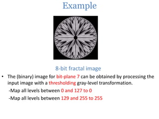
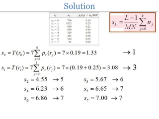
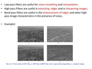
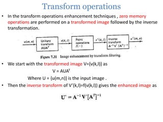
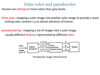
![Point operations
-Zero-memory operations where a given gray level u∈[0,L] is mapped
into a gray level v∈[0,L] according to a transformation.
v(m,n)=f(u(m,n))](https://image.slidesharecdn.com/imageenhancement-140107041340-phpapp02/85/Image-enhancement-6-320.jpg)

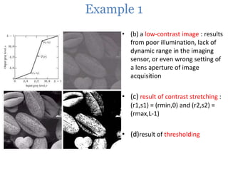

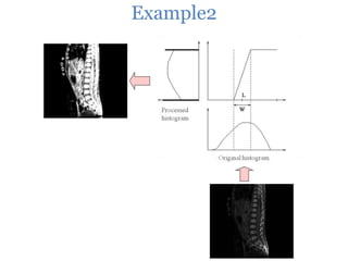
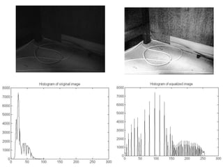
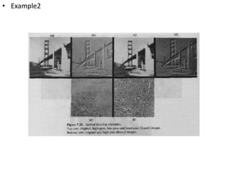
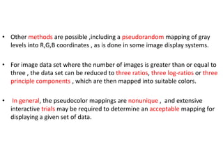
![2-Clipping and Thresholding
• Expressed as :
• Clipping:
-Special case of contrast stretching ,where α= γ=0
-Useful for noise reduction when the input signal is known to lie in the
range [a,b].](https://image.slidesharecdn.com/imageenhancement-140107041340-phpapp02/85/Image-enhancement-10-320.jpg)


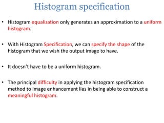


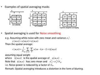
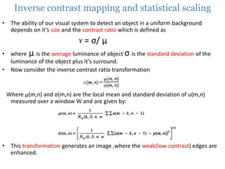
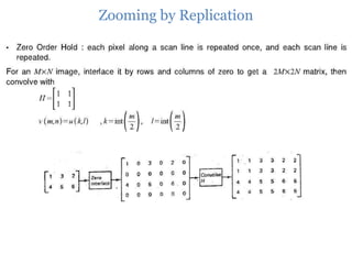
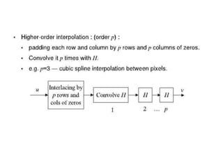
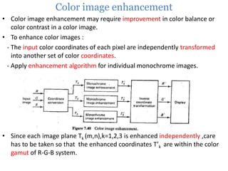
![Spatial operations
• Operations performed on local neighborhoods of input pixels
• Image is convolved with [FIR] finite impulse response filter called
spatial mask .
• Techniques such as :
- Noise smoothing
- Median filtering
- LP,HP &PB filtering
- Zooming](https://image.slidesharecdn.com/imageenhancement-140107041340-phpapp02/85/Image-enhancement-35-320.jpg)


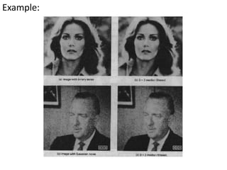
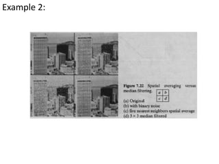
![Median filtering
• Input pixel is replaced by the median of the pixels contained in a window
around a pixel
• The algorithm requires arranging the pixels in an increasing or decreasing
order and picking the middle value.
• For Odd window size is commonly used [3*3-5*5-7*7]
• For even window size the average of two middle values is taken.
• Median filter properties:
1- Non-linear filter
2-Performes very well on images containing binary noise , poorly when the
noise is gaussian.
3-performance is poor in case that the number of noise pixels in the window is
greater than or half the number of pixels in the window.](https://image.slidesharecdn.com/imageenhancement-140107041340-phpapp02/85/Image-enhancement-40-320.jpg)


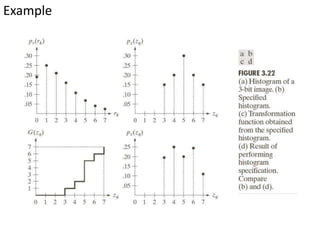
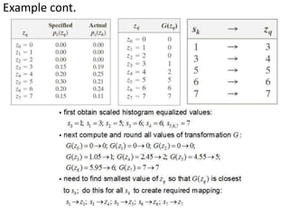
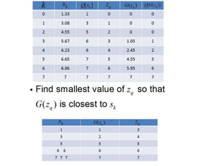
This document provides an overview of various image enhancement techniques. It begins with an introduction to image enhancement and its objectives. It then outlines and describes several categories of enhancement methods, including spatial-frequency domain methods, point operations, histogram operations, spatial operations, and transform operations. Specific techniques discussed in detail include contrast stretching, clipping, thresholding, median filtering, unsharp masking, and principal component analysis for multispectral images. The document also covers color image enhancement and techniques for pseudocoloring.


![5G Explained! A High Level Overview [Introduction]](https://cdn.slidesharecdn.com/ss_thumbnails/5gexplainedahighleveloverview-260119165306-cc137a3e-thumbnail.jpg?width=640&height=640&fit=bounds)


