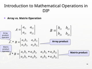
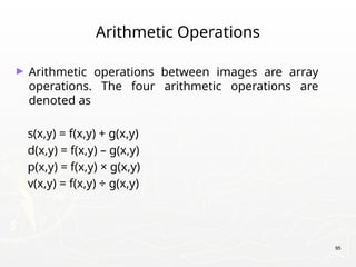
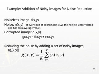
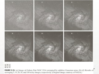
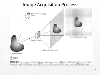
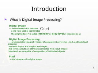
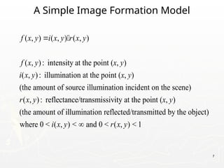
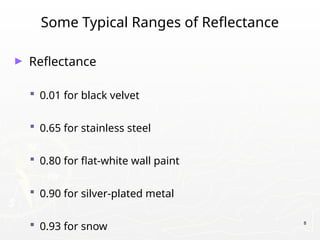
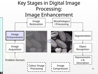
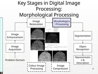
The document provides an introduction to digital image processing, explaining concepts such as image representation, sampling, quantization, and key stages in processing. It covers various types of digital images, techniques used for image enhancement, restoration, and segmentation, and highlights applications in fields like biometrics and autonomous vehicles. Additionally, it discusses essential relationships between pixels and mathematical operations pertaining to image processing.

![19
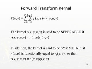
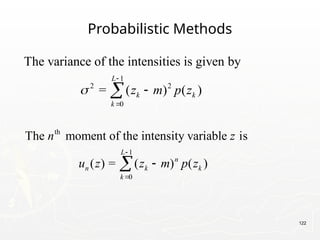
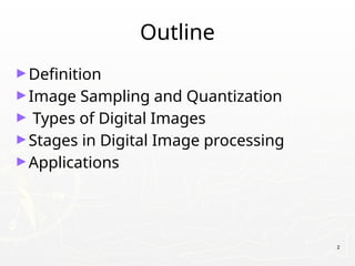
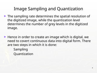
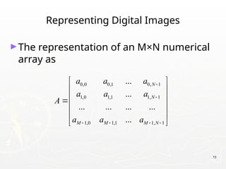
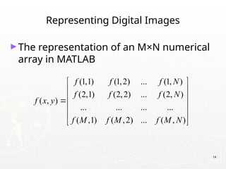
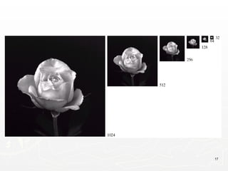
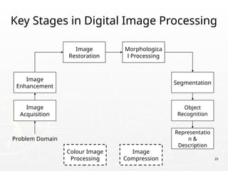
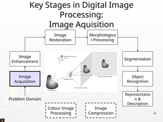
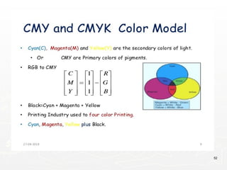
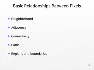
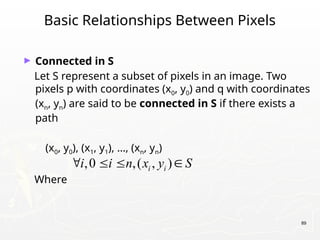
Representing Digital Images
► Discrete intensity interval [0, L-1], L=2k
► The number b of bits required to store a M × N
digitized image
b = M × N × k](https://image.slidesharecdn.com/unit1fullnotesslo-241019164900-7564e508/85/Digital-Image-Processing-Unit-1-NotesPPT-19-320.jpg)


![92
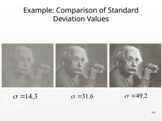
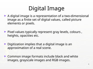
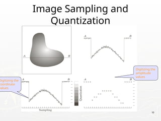
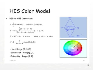
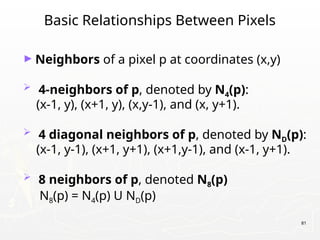
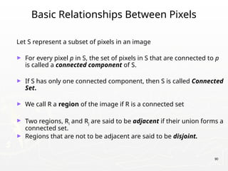
Distance Measures
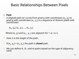
► Given pixels p, q and z with coordinates (x, y), (s, t),
(u, v) respectively, the distance function D has
following properties:
a. D(p, q) 0 [D(p, q) = 0, iff p = q]
≥
b. D(p, q) = D(q, p)
c. D(p, z) D(p, q) + D(q, z)
≤](https://image.slidesharecdn.com/unit1fullnotesslo-241019164900-7564e508/85/Digital-Image-Processing-Unit-1-NotesPPT-92-320.jpg)
![93
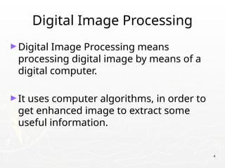
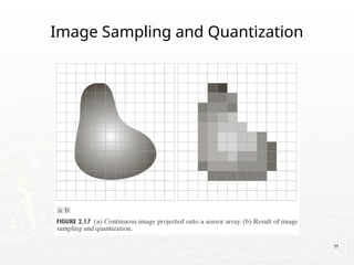
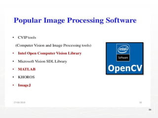
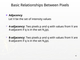
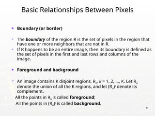
Distance Measures
The following are the different Distance measures:
a. Euclidean Distance :
De(p, q) = [(x-s)2
+ (y-t)2
]1/2
b. City Block Distance:
D4(p, q) = |x-s| + |y-t|
c. Chess Board Distance:
D8(p, q) = max(|x-s|, |y-t|)](https://image.slidesharecdn.com/unit1fullnotesslo-241019164900-7564e508/85/Digital-Image-Processing-Unit-1-NotesPPT-93-320.jpg)