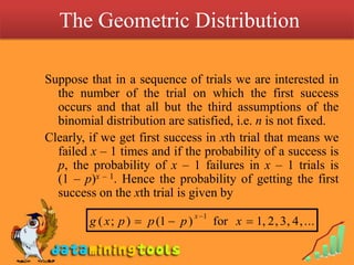
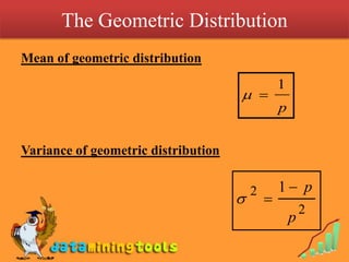
1.12 Poisson Distribution, Poisson Process & Geometric Distribution
The Poisson DistributionPoisson Distribution: A random variable X is said to have a Poisson distribution with mean , if its density function is given by:
Since the infinite series in the expression on the right is Maclaurin’s series for e, it follows thatTo verify P(S) = 1 for Poisson distribution formula
Proof 1
Moment Generating function for Poisson distribution
Moment Generating function for Poisson distributionMoment Generating function for Poisson distribution
Moment Generating function for Poisson distribution
The Poisson Approximation to the Binomial Distribution To Show that when n  and p  0, while np =  remain constant, b(x;n,p)  f(x; ).Proof: First we substitute /n for p into the formula for the binomial distribution, we get
The Poisson Approximation to the Binomial Distribution If n, we have
The Poisson Approximation to the Binomial Distribution andHencePoisson distribution function:
The Poisson Approximation to the Binomial Distribution Table 2 at the end of the book gives the value of Poisson distribution function F(x; ) for values of  in varying increments from up to 15, and its use is very similar to that of Table 1.The value of f(x;) can be obtained by formulaf(x; ) = F(x; ) - F(x - 1; )An acceptable rule of thumb is to use Poisson approximation to the binomial distribution if n  20 and p  0.05; if n  100, the approximation is generally excellent so long as np  10.
Poisson Processes Suppose we are concerned with discrete events taking place over continuous intervals (not in the usual mathematical sense) of time, length or space; such as the arrival of telephone calls at a switchboard, or number of red blood cells in a drop of blood (here the continuous interval involved is a drop of blood).To find the probability of x successes during a time interval of length T we divide the interval into n equal parts of length t , so that T  = n  t, and we assume that:
Poisson Processes 1. The probability of a success during a very small interval of time t is given by  . t.2. The probability of more than one success during such a small time interval t is negligible.3. The probability of success in non-overlapping intervals t are independent.
Poisson Processes This means that assumptions for the binomial distribution are satisfied and the probability of x successes in the time interval T is given by the binomial probability b(x; n, p) with n = T / t and p =  . t.When n   the probability of x successes during the time interval T  is given by the corresponding Poisson probability f(x; ) with the parameter
Poisson Processes Since  is the mean of this Poisson distribution, note that  is the average (mean) number of successes per unit time.The Poisson distribution has many important applications in queuing problems, where we may be interested, for example, in number of customers arriving for service at a cafeteria, the number of ships or trucks arriving to be unloaded at a receiving dock, the number of aircrafts arriving at an airport and so forth.
 The Geometric DistributionSuppose that in a sequence of trials we are interested in the number of the trial on which the first success occurs and that all but the third assumptions of the binomial distribution are satisfied, i.e. n is not fixed.Clearly, if we get first success in xth trial that means we failed x – 1 times and if the probability of a success is p, the probability of x – 1 failures in x – 1 trials is      (1 – p)x – 1. Hence the probability of getting the first success on the xth trial is given by
The Geometric DistributionMean of geometric distributionVariance of geometric distribution

Poisson Distribution, Poisson Process & Geometric Distribution

  • 1.
    1.12 Poisson Distribution,Poisson Process & Geometric Distribution
  • 2.
    The Poisson DistributionPoissonDistribution: A random variable X is said to have a Poisson distribution with mean , if its density function is given by:
  • 3.
    Since the infiniteseries in the expression on the right is Maclaurin’s series for e, it follows thatTo verify P(S) = 1 for Poisson distribution formula
  • 4.
  • 7.
    Moment Generating functionfor Poisson distribution
  • 8.
    Moment Generating functionfor Poisson distributionMoment Generating function for Poisson distribution
  • 9.
    Moment Generating functionfor Poisson distribution
  • 10.
    The Poisson Approximationto the Binomial Distribution To Show that when n  and p  0, while np =  remain constant, b(x;n,p)  f(x; ).Proof: First we substitute /n for p into the formula for the binomial distribution, we get
  • 11.
    The Poisson Approximationto the Binomial Distribution If n, we have
  • 12.
    The Poisson Approximationto the Binomial Distribution andHencePoisson distribution function:
  • 13.
    The Poisson Approximationto the Binomial Distribution Table 2 at the end of the book gives the value of Poisson distribution function F(x; ) for values of  in varying increments from up to 15, and its use is very similar to that of Table 1.The value of f(x;) can be obtained by formulaf(x; ) = F(x; ) - F(x - 1; )An acceptable rule of thumb is to use Poisson approximation to the binomial distribution if n  20 and p  0.05; if n  100, the approximation is generally excellent so long as np  10.
  • 14.
    Poisson Processes Supposewe are concerned with discrete events taking place over continuous intervals (not in the usual mathematical sense) of time, length or space; such as the arrival of telephone calls at a switchboard, or number of red blood cells in a drop of blood (here the continuous interval involved is a drop of blood).To find the probability of x successes during a time interval of length T we divide the interval into n equal parts of length t , so that T = n  t, and we assume that:
  • 15.
    Poisson Processes 1.The probability of a success during a very small interval of time t is given by  . t.2. The probability of more than one success during such a small time interval t is negligible.3. The probability of success in non-overlapping intervals t are independent.
  • 16.
    Poisson Processes Thismeans that assumptions for the binomial distribution are satisfied and the probability of x successes in the time interval T is given by the binomial probability b(x; n, p) with n = T / t and p =  . t.When n   the probability of x successes during the time interval T is given by the corresponding Poisson probability f(x; ) with the parameter
  • 17.
    Poisson Processes Since is the mean of this Poisson distribution, note that  is the average (mean) number of successes per unit time.The Poisson distribution has many important applications in queuing problems, where we may be interested, for example, in number of customers arriving for service at a cafeteria, the number of ships or trucks arriving to be unloaded at a receiving dock, the number of aircrafts arriving at an airport and so forth.
  • 18.
    The GeometricDistributionSuppose that in a sequence of trials we are interested in the number of the trial on which the first success occurs and that all but the third assumptions of the binomial distribution are satisfied, i.e. n is not fixed.Clearly, if we get first success in xth trial that means we failed x – 1 times and if the probability of a success is p, the probability of x – 1 failures in x – 1 trials is (1 – p)x – 1. Hence the probability of getting the first success on the xth trial is given by
  • 19.
    The Geometric DistributionMeanof geometric distributionVariance of geometric distribution