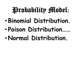
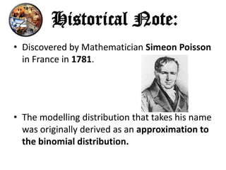
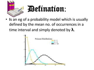
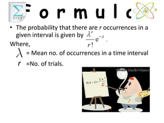
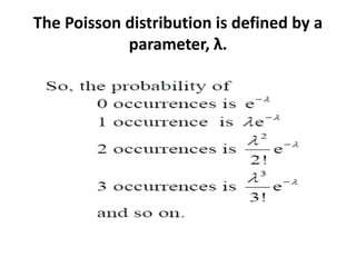
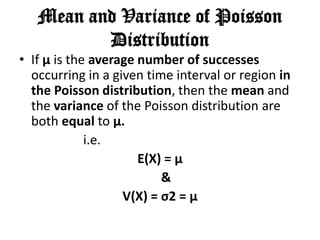
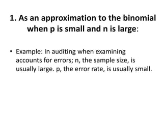
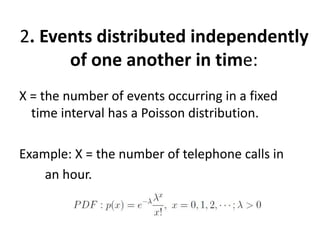
This document discusses three probability distributions: the binomial, Poisson, and normal distributions. It provides details on the Poisson distribution, including its definition as a model for independent and random events with a constant probability over time. Examples are given of how the Poisson distribution can model the number of occurrences in a fixed time period, such as telephone calls in an hour. The key properties of the Poisson distribution are that the mean and variance are equal to the parameter lambda.

2. Probability Model:
• Binomial
Distribution…….
• Poison Distribution
• Normal Distribution.

3. The Binomial Distribution…...

4. Defination:

5. Examples:

6. Examples::

7. Examples:::

21. Probability Model:
• Binomial Distribution.
• Poison Distribution……
• Normal Distribution.

22. POISSON
DISTRIBUTION…….

23. Historical Note:
• Discovered by Mathematician Simeon Poisson
in France in 1781.
• The modelling distribution that takes his name
was originally derived as an approximation to
the binomial distribution.

24. Defination:
• Is an eg of a probability model which is usually
defined by the mean no. of occurrences in a
time interval and simply denoted by λ.

25. Uses:
• Occurrences are independent.
• Occurrences are random.
• The probability of an occurrence is constant
over time.

26. Sum of two Poisson
distributions:
• If two independent random variables both
have Poisson distributions with parameters λ
and μ, then their sum also has a Poisson
distribution and its parameter is λ + μ .

27. The Poisson distribution may be used to model a
binomial distribution, B(n, p) provided that
• n is large.
• p is small.
• np is not too large.

28. F o r m u l a:
• The probability that there are r occurrences in a
given interval is given by
Where,
= Mean no. of occurrences in a time interval
r =No. of trials.

29. The Poisson distribution is defined by a
parameter, λ.

30. Mean and Variance of Poisson
Distribution
• If μ is the average number of successes
occurring in a given time interval or region in
the Poisson distribution, then the mean and
the variance of the Poisson distribution are
both equal to μ.
i.e.
E(X) = μ
&
V(X) = σ2 = μ

31. Examples:
1. Number of telephone calls in a week.
2. Number of people arriving at a checkout in a
day.
3. Number of industrial accidents per month in a
manufacturing plant.

32. Graph :
• Let’s continue to assume we have a
continuous variable x and graph the Poisson
Distribution, it will be a continuous curve, as
follows:
Fig: Poison distribution graph.

33. Example:
Twenty sheets of aluminum alloy were examined for surface
flaws. The frequency of the number of sheets with a given
number of flaws per sheet was as follows:
What is the probability of finding a sheet chosen
at random which contains 3 or more surface
flaws?

34. Generally,
• X = number of events, distributed
independently in time, occurring in a fixed
time interval.
• X is a Poisson variable with pdf:
• where is the average.

35. Application:
• The Poisson distribution arises in two ways:

36. 1. As an approximation to the binomial
when p is small and n is large:
• Example: In auditing when examining
accounts for errors; n, the sample size, is
usually large. p, the error rate, is usually small.

37. 2. Events distributed independently
of one another in time:
X = the number of events occurring in a fixed
time interval has a Poisson distribution.
Example: X = the number of telephone calls in
an hour.

39. Probability Model:
• Binomial Distribution.
• Poison Distribution
• Normal
Distribution…….

40. The Normal Distribution…...

53. •The End

54. Thank You….