UNIT-3 network security layers andits types

Syllabus
Network Layer Services – Packet switching –
Performance – IPV4 Addresses – Forwarding
of IP Packets - Network Layer Protocols: IP,
ICMP v4 – Unicast Routing Algorithms –
Protocols – Multicasting Basics – IPV6
Addressing – IPV6 Protocol.

Network Layer Services (Network layer duties)
The key is interconnecting different networks (various
LAN technologies, telephone network, satellite link,
ATM networks etc.)

Network layer duties
• The addresses must be uniquely and universally define the
sole connection of a (host/router/machine/device/user) to the
internet.
•Two devices on the internet can never have the same
address. (Address per connection)

• Network layer encapsulates packets received from upper
layer protocols and makes new packets. (Re-packaging).
• In the Internet model, packetizing is done by network layer
protocol called IP – Internetworking Protocol.
• The Protocol Data Units (PDU’s) coming from the transport
layer must be placed in network-layer packets and sent to
the data-link layer.

Packetizing
•The first duty of the network layer is definitely packetizing:
encapsulating the payload (data received from upper layer)
in a network-layer packet at the source and decapsulating
the payload from the network-layer packet at the destination.
•The source host receives the payload from an upper-layer
protocol, adds a header that contains the source and
destination addresses and some other information that is
required by the network-layer protocol and delivers the
packet to the data-link layer.
•The destination host receives the network-layer packet
from its data-link layer, decapsulates the packet, and
delivers the payload to the corresponding upper-layer
protocol.

7
• A packet can travel through different networks.
• Each router decapsulates the IP datagram from the received
frame, processes it and then encapsulates it in another frame.
• The format & size depend on the physical network.
• The network layer must be able to fragment transport layer PDUs
into smaller units so that they can be transferred over various data-
link layer technologies.

Fragmentation
• If the packet is fragmented at the source or at
routers along the path, the network layer is
responsible for waiting until all fragments
arrive, reassembling them, and delivering
them to the upper-layer protocol.

• Now that you have your network layer packet, where
do you send it ? Each packet reaches its destination via
several routes.
• So, which route is suitable or optimum? Issue of
speed, reliability, security etc. (routing algorithm)
• Packet cannot choose the route; the routers
connecting the LANs/WANs makes this decision.

Routing and Forwarding
Routing
• The network layer is responsible for routing the packet
from its source to the destination.
• A physical network is a combination of networks (LANs
and WANs) and routers that connect them.
• The network layer is responsible for finding the best
one among these possible routes.
• The network layer needs to have some specific
strategies for defining the best route.
• In the Internet today, this is done by running some
routing protocols to help the routers coordinate their
knowledge about the neighbourhood and to come up
with consistent tables to be used when a packet
arrives.

Forwarding
• If routing is applying strategies and running some routing protocols to create the
decision-making tables for each router, forwarding can be defined as the action
applied by each router when a packet arrives at one of its interfaces.
• The decision-making table a router normally uses for applying this action is
sometimes called the forwarding table and sometimes the routing table.
• When a router receives a packet from one of its attached networks, it needs to
forward the packet to another attached network (in unicast routing) or to some
attached networks (in multicast routing).
• To make this decision, the router uses a piece of information in the packet header,
which can be the destination address or a label, to find the corresponding output
interface number in the forwarding table.

• As the figure shows, the network layer is involved at the
source host, destination host, and all routers in the path
(R2, R4, R5, and R7).
• At the source host (Alice), the network layer accepts a
packet from a transport layer, encapsulates the packet in a
datagram, and delivers the packet to the data-link layer.
• At the destination host (Bob), the datagram is
decapsulated, and the packet is extracted and delivered to
the corresponding transport layer.
• Although the source and destination hosts are involved in
all five layers of the TCP/IP suite, the routers use three
layers if they are routing packets only; however, they may
need the transport and application layers for control
purposes.
• A router in the path is normally shown with two data-link
layers and two physical layers, because it receives a packet
from one network and delivers it to another network.

Other Services
Error Control
• Although the network layer in the Internet does not directly provide error
control, the Internet uses an auxiliary protocol, ICMP that provides some kind of
error control if the datagram is discarded or has some unknown information in
the header.
• Flow control regulates the amount of data a source can send without
overwhelming the receiver.
• To control the flow of data, the receiver needs to send some feedback to the
sender to inform the latter that it is overwhelmed with data.
• The network layer in the Internet, however, does not directly provide any flow
control.
Congestion Control
• Another issue in a network-layer protocol is congestion control.
• Congestion in the network layer is a situation in which too many data grams are
present in an area of the Internet.
• Congestion may occur if the number of data grams sent by source computers is
beyond the capacity of the network or routers. If the congestion continues,
sometimes a situation may reach a point where the system collapses and no data
grams are delivered.

Quality of Service
• As the Internet has allowed new applications such as multimedia
communication (in particular real-time communication of audio and
video), the quality of service (QoS) of the communication has
become more and more important.
• The Internet has thrived by providing better quality of service to
support these applications.
Security
• Another issue related to communication at the network layer is
security.
• The network layer was designed with no security provision. Today,
however, security is a big concern.
• To provide security for a connectionless network layer, we need to
have another virtual level that changes the connectionless service
to a connection-oriented service.

NETWORK-LAYER PERFORMANCE
• The performance of a network can be measured in terms of delay,
throughput, and packet loss.
• Congestion control is an issue that can improve the performance.
Delay
• The delays in a network can be divided into four types: transmission delay,
propagation delay, processing delay, and queuing delay.
Transmission Delay
• A source host or a router cannot send a packet instantaneously. A sender
needs to put the bits in a packet on the line one by one. If the first bit of the
packet is put on the line at time t1 and the last bit is put on the line at time
t2, transmission delay of the packet is (t2 −t1). So the transmission delay is
Delaytr = (Packet length) / (Transmission rate)
• For example, in a Fast Ethernet LAN with the transmission rate of 100
million bits per second and a packet of 10,000 bits, it takes
(10,000)/(100,000,000) or 100 microseconds for all bits of the packet to be
put on the line.

Propagation Delay
• Propagation delay is the time it takes for a bit to travel from point A to
point B in the transmission media.
• The propagation delay depends on the propagation speed of the media,
which is 3×108 meters/second in a vacuum and normally much less in a
wired medium; it also depends on the distance of the link.
• In other words, propagation delay is
Delaypg= (Distance) / (Propagation speed).
• For example, if the distances of a cable link in a point-to-point WAN is
2000 meters and the propagation speed of the bits in the cable is 2×108
meters/second, then the propagation delay is 10 microseconds.
Processing Delay
• The processing delay is the time required for a destination host to receive
a packet from its input port, remove the header, perform an error
detection procedure, and deliver the packet to the output port.
• The processing delay may be different for each packet, but normally is
calculated as an average.
Delaypr =Time required to process a packet in a router or a destination
host

Queuing Delay
• Queuing delay can normally happen in a router.
• The queuing delay for a packet in a router is measured as the time a
packet waits in the input queue and output queue of a router.
Delayqu =The time a packet waits in input and output queues in a
router
Total Delay
• Assuming equal delays for the sender, routers, and receiver, the total
delay (source-to destination delay) a packet encounters can be
calculated if we know the number of routers, n, in the whole path.
Total delay = (n +1) (Delaytr +Delaypg +Delaypr) + (n) (Delayqu)
• Note that if we have n routers, we have (n +1) links. Therefore, we have
(n +1) transmission delays related to n routers and the source, (n +1)
propagation delays related to (n +1) links, (n +1) processing delays
related to n routers and the destination, and only n queuing delays
related to n routers.

Throughput
• Throughput at any point in a network is defined as the number of
bits passing through the point in a second, which is actually the
transmission rate of data at that point.
• In a path from source to destination, a packet may pass through
several links (networks), each with a different transmission rate.
• In this figure, the data can flow at the rate of 200 kbps in Link1.
However, when the data arrives at router R1, it cannot pass at this
rate. Data needs to be queued at the router and sent at 100 kbps.
When data arrives at router R2, it could be sent at the rate of 150
kbps, but there is not enough data to be sent.
Figure . Throughput in a path with three links in a series

• In other words, the average rate of the data flow in Link3 is also 100 kbps.
• We can conclude that the average data rate for this path is 100 kbps, the
minimum of the three different data rates.
• We can simulate the behaviour of each link with pipes of different sizes;
the average throughput is determined by the bottleneck, the pipe with
the smallest diameter.
• In general, in a path with n links in series, we have
Throughput = minimum {TR1, TR2 ...TRn}.
• Although the situation in above figure shows how to calculate the
throughput when the data is passed through several links, the actual
situation in the Internet is that the data normally passes through two
access networks and the Internet backbone, as shown in the below
Figure.

• Figure shows this situation, in which the throughput is the
minimum of TR1 and TR2.
• For example, if a server connects to the Internet via a Fast
Ethernet LAN with the data rate of 100 Mbps, but a user who
wants to download a file connects to the Internet via a dial-up
telephone line with the data rate of 40 kbps, the throughput is
40 kbps. The bottleneck is definitely the dial-up line.
• In the below figure, transmission rate of the link between the
two routers is actually shared between the flows and this
should be considered when we calculate the throughput.
• For example, in Figure the transmission rate of the main link in
the calculation of the throughput is only 200 kbps because the
link is shared between three paths.

Packet Loss
• Another issue that severely affects the performance of
communication is the number of packets lost during
transmission.
• When a router receives a packet while processing another
packet, the received packet needs to be stored in the input
buffer waiting for its turn.
• A router, however, has an input buffer with a limited size. A
time may come when the buffer is full and the next packet
needs to be dropped.
• The effect of packet loss on the Internet network layer is
that the packet needs to be resent, which in turn may
create overflow and cause more packet loss.

24.23
CONGESTION
Congestion in a network may occur if the load on
the network—the number of packets sent to the network
is greater than the capacity of the network—the number
of packets a network can handle.
Congestion control refers to the mechanisms and
techniques to control the congestion and keep the load
below the capacity.

24.24
CONGESTION CONTROL
Congestion control refers to techniques and
mechanisms that can either prevent congestion, before it
happens, or remove congestion, after it has happened.
In general, we can divide congestion control
mechanisms into two broad categories:
open-loop congestion control (prevention)
closed-loop congestion control (removal)

24.25
Congestion control categories

1. Open-Loop Congestion Control
In open-loop congestion control, policies are applied to prevent congestion before it
happens.
1.1 Retransmission Policy
If the sender feels that a sent packet is lost or corrupted, the packet needs to be
retransmitted.
The retransmission policy and the retransmission timers must be designed to optimize
efficiency and at the same time prevent congestion.
1.2 Window Policy
The type of window at the sender may also affect congestion.
The Selective Repeat window is better than the Go-Back-N window for congestion
control.
1.3 Acknowledgment Policy
The acknowledgment policy imposed by the receiver may also affect congestion.
Sending fewer acknowledgments means imposing fewer loads on the network.
24.26

1.4 Discarding Policy
A good discarding policy by the routers may prevent congestion and at
the same time may not harm the integrity of the transmission.
1.5Admission Policy
An admission policy, which is a quality-of-service mechanism, can also
prevent congestion in virtual-circuit networks.
24.27

2. Closed-Loop Congestion Control
Closed-loop congestion control mechanisms try to alleviate
congestion after it happens.
2.1 Backpressure
Backpressure is a node-to-node congestion control that starts
with a node and propagates, in the opposite direction of data
flow, to the source.
24.28

2.2 Choke packet
A choke packet is a packet sent by a node to the source to inform it of
congestion.
In backpressure, the warning is from one node to its upstream node,
although the warning may eventually reach the source station.
In the choke packet method, the warning is from the router, which has
encountered congestion, to the source station directly.
24.29

2.3 Implicit Signaling
In implicit signaling, there is no communication between the congested node
or nodes and the source.
The source guesses that there is congestion somewhere in the network from
other symptoms.
2.4 Explicit Signaling
The node that experiences congestion can explicitly send a signal to the
source or destination. In the choke packet method, a separate packet is used
for this purpose; in the explicit signaling method, the signal is included in the
packets that carry data.
(i)Backward Signaling-A bit can be set in a packet moving in the direction
opposite to the congestion.
This bit can warn the source that there is congestion and that it needs to slow
down to avoid the discarding of packets.
(ii)Forward Signaling-A bit can be set in a packet moving in the direction of the
congestion.
This bit can warn the destination that there is congestion.
24.30

IP Addressing (IPV4 Addresses)
1. Every host and router on the internet is provided with a unique address, which encodes its network number
and host number.
2. No two nodes have the same IP addresses.
3. The IP addresses are 32-bit long having the formats shown in Fig.3.11. The three main address formats are
assigned with network addresses (net id) and host address (host id) fields of different sizes.
4. The class A format allows up to 126 networks with 16 million hosts each.
5. Class B allows up to 16,382 networks with up to 64 K hosts each.
6. Class C allows 2 million networks with up to 254 hosts each.
7. The Class D is used for multicasting in which a datagram is directed to multiple hosts.
8. Addresses beginning with 11110 are reserved for future use.
Fig.3.11 IP address formats

1. Network addresses are usually written in dotted decimal notation, such as 128.11.3.31 as in Fig.3.13.
2. Range of IP addresses for different classes is given in Fig.3.12. This approach of representing IP addresses
in terms of classes is known as classful addressing.
3. In mid 90’s another approach known as classless addressing has been proposed, which may replace the
existing classful addressing approach in future.
Fig.3.12 Range of IP addresses for different classes
Notations
There are two notations to show an IPv4 address:
1. Binary notation
2. Dotted- decimal notation.
Fig.3.13 Dotted decimal representation

Example 1
Change the following IP addresses from binary notation to
dotted-decimal notation.
a. 10000001 00001011 00001011 11101111
b. 11111001 10011011 11111011 00001111
Solution
We replace each group of 8 bits with its equivalent decimal
number and add dots for separation:
a. 129.11.11.239
b. 249.155.251.15

Example 2
Change the following IP addresses from dotted-decimal
notation to binary notation.
a. 111.56.45.78
b. 75.45.34.78
Solution
We replace each decimal number with its binary equivalent :
a. 01101111 00111000 00101101 01001110
b. 01001011 00101101 00100010 01001110

Find the class of each address.
a. 00000001 00001011 00001011 11101111
b. 11000001 10000011 00011011 11111111
c. 14.23.120.8
d. 252.5.15.111
Solution
a. The first bit is 0. This is a class A address.
b. The first 2 bits are 1; the third bit is 0. This is a class C
address.
c. The first byte is 14; the class is A.
d. The first byte is 252; the class is E.
Example 3

Classful Addressing
a) Unicast address: one source to one destination; Class A, B & C.
b) Multicast address: one source to a group of destination: only as
destination address not source address; Class-D.
c) IP addresses in class A, B, C are divided into different length of:
Network-ID (netid) and Host-ID (hostid)
d) Classes and Blocks concept: - for example:
In class-A, 1st block covers from 0.0.0.0 to 0.255.255.255 (net-ID 0)
2nd block covers from 1.0.0.0 to 1.255.255.255 (net-ID 1)
last block covers from 127.0.0.0 to 127.255.255.255 (net-ID 127)
• Note that: block = number of available networks in each class
• One problem with classful addressing is that each class is
divided into a fixed number of blocks with fixed size.
• Plenty of IP addresses wasted!!! in classful addressing method.

37
128 Blocks in class A
1st IP used to identify organisation
to the rest of Internet
Last IP reserved for special
purpose; not allowed to use
Millions of class A addresses are wasted.
3 bytes
= 224

38
16384 Blocks in class B
Many of class B addresses are wasted.
Class B for midsize organisation.
16384 organizations are class-B
16 blocks for private addressees
leaving 16368 blocks

2,097,152 Blocks in class C
256 blocks for private addressees
leaving 2,096,896 blocks
Class C for small organisation.
Limited IP address in each blocks,
which is smaller than the needs of
most organisations

Class D addresses
are used for multicasting;
there is only
one block in this class.
Class E addresses are reserved
for special purposes;
most of the block is wasted.

Sub netting
1. To filter packets for a particular network, a router uses a concept known
as masking, which filters out the net id part (by ANDing with all 1’s) by
removing the host id part (by ANDing with all 0’s).
2. All the hosts in a network must have the same network number. This
property of IP addressing causes problem as the network grows.
3. To overcome this problem, a concept known as subnets is used, which
splits a network into several parts for internal use, but still acts like a
single network to the outside world.
4. To facilitate routing, a concept known as subnet mask is used. Mask can
help us to find the netid and hostid.
5. It is 32-bit number made of contiguous1s followed by contiguous 0s.
Super netting
1. In super netting, an organization can combine several class C blocks to
create a larger range of addresses.
2. Several networks are combined to create a super network (super net).

Classless Addressing
• Sub netting and super netting in classful addressing did not really
solve the address depletion problem.
• The larger address space, however, requires that the length of IP
addresses also be increased, which means the format of the IP
packets needs to be changed.
• long-range solution is IPv6, a short-term solution was also devised
to use the same address space but to change the distribution of
addresses to provide a fair share to each organization.
• The short-term solution still uses IPv4 addresses, but it is called
classless addressing.

• In classless addressing, variable-length blocks are used that
belong to no classes.
• We can have a block of 1 address, 2 addresses, 4 addresses, 128
addresses, and so on.
• In classless addressing, the whole address space is divided into
variable length blocks. The prefix in an address defines the block
(network); the suffix defines the node (device).
• Theoretically, we can have a block of 20, 21, 22…232 addresses.
• One of the restrictions is that the number of addresses in a block
needs to be a power of 2.
• An organization can be granted one block of addresses. Figure
shows the division of the whole address space into
nonoverlapping blocks.

• Unlike classful addressing, the prefix length in
classless addressing is variable. We can have a
prefix length that ranges from 0 to 32.
• Since the prefix length is not inherent in the
address, we need to separately give the length
of the prefix.
• In this case, the prefix length, n, is added to
the address, separated by a slash.
• The notation is informally referred to as slash
notation and formally as classless
interdomain routing or CIDR (pronounced
cider) strategy

Extracting Information from an Address
• Given any address in the block, we normally like to know three pieces of
information about the block to which the address belongs: the number of
addresses, the first address in the block, and the last address.
• Since the value of prefix length, n, is given, we can easily find these three
pieces of information, as shown in Figure.
1. The number of addresses in the block is found as N = 232-n.
2. To find the first address, we keep the n leftmost bits and set the (32 - n)
rightmost bits all to 0s.
3. To find the last address, we keep the n leftmost bits and set the (32 - n)
rightmost bits all to 1s.

Example
• A classless address is given as 167.199.170.82/27. We can find the above
three pieces of information as follows.
1. The number of addresses in the network is 232-n= 25 = 32 addresses.
2. The first address can be found by keeping the first 27 bits and changing the
rest of the bits to 0s.
Address: 167.199.170.82/27
10100111 11000111 10101010 01010010
First address: 167.199.170.64/27
10100111 11000111 10101010 01000000
3. The last address can be found by keeping the first 27 bits and changing the
rest of the bits to 1s.
Address: 167.199.170.82/27
10100111 11000111 10101010 01011111
Last address: 167.199.170.95/27
10100111 11000111 10101010 01011111

Mask
A mask is a 32-bit binary number or 4-bytes that gives the first address in the block
(the network address) when bitwise ANDed with an address in the block.

48
Default Mask for classful addressing
CIDR (Classless Interdomain Routing) or slash notation:
It is used to show the mask in the form /n (n=8, 16, 24).

Fig.3.14 Masking with the help of router
Fig.3.15 Subnet masking with the help of router

Example-6
Given the address 23.56.7.91 and the default class A
mask, find the beginning address (network address).
Solution
The default mask is 255.0.0.0, which means that only
the first byte is preserved and the other 3 bytes are set
to 0s. The network address is 23.0.0.0.

Example-7
Given the address 132.6.17.85 and the default class B
mask, find network address.
Solution
The default mask is 255.255.0.0, which means that the first
2 bytes are preserved and the other 2 bytes are set to 0s.
The network address is 132.6.0.0.

Example-8
Given the address 201.180.56.5 and the class C
default mask, find the network address.
Solution
The default mask is 255.255.255.0, which means that the
first 3 bytes are preserved and the last byte is set to 0. The
network address is 201.180.56.0.

Example-9
What is the sub-network address if the destination address
is 19.30.84.5 and the mask is 255.255.192.0?
Solution Answer: Subnet Address = 19.30.64.0

Example
A company is granted the site address 201.70.64.0 (class C). The
company needs six subnets. Design the subnets.
Solution
The number of 1s in the default mask is 24 (class C).
The company needs six subnets. Since 6 is not a power of 2, the next
number that is a power of 2 is 8 (23). That means up to 8 subnets.
Hence, we need 3 more ‘1’s in the subnet mask =
11111111.11111111.11111111.11100000 or 255.255.255.224
The total number of 1s in the subnet mask is 27 (24 + 3).
Since the total number of 0s is 5 (32 - 27).
The number of addresses in each subnet is 25 (5 is the
number of 0s) or 32.

subnets are :
201.70.64.0
201.70.64.32
201.70.64.64
201.70.64.96
201.70.64.128
201.70.64.160
201.70.64.192
201.70.64.224

Example
Solution
A company is granted the site address 181.56.0.0 (class B). The company
needs 1000 subnets. Design the subnets.
The number of 1s in the default mask is 16 (class B).
The company needs 1000 subnets. This number is not a power of 2. The next
number that is a power of 2 is 1024 (210). We need 10 more 1s in the subnet
mask.
The total number of 1s in the subnet mask is 26 (16 + 10).
The total number of 0s is 6 (32 − 26).
The mask is
11111111 11111111 11111111 11000000
or
255.255.255.192.
The number of subnets is 1024.
The number of addresses in each subnet is 26 (6 is the number of 0s) or 64.

http://osnet.cs.nchu.edu.tw/powpoint/netwo
rk/Chapter%205.pdf

Addresses in a network
With and without sub netting
Just like telephone system

Network Addresses
• The network address is the first address.
• The network address defines the network to
the rest of the Internet.
• Given the network address, we can find the
class of the address, the block, and the range of
the addresses in the block.

Network addresses
In classful addressing, the network address
(the first address in the block)
is the one that is assigned to the organization.

Given the address 23.56.7.91, find the network address.
Solution:
The class is A. Only the first byte defines the netid. We can find the
network address by replacing the hostid bytes (56.7.91) with 0s.
Therefore, the network address is 23.0.0.0.
Given the address
132.6.17.85 and 23.56.7.91, find the network address?
Solution
1. The class is B. The first 2 bytes defines the netid. We can find the network
address by replacing the hostid bytes (17.85) with 0s. 132.6.0.0.
2. The class is A. Only the first byte defines the netid. We can find the
network address by replacing the hostid bytes (56.7.91) with 0s.
Therefore, the network address is 23.0.0.0.
Example
Example

Hierarchy
• IP addresses have levels of hierarchy. For example, a telephone network in North America
has three levels of hierarchy.
• The leftmost three digits define the area code, the next three digits define the exchange, the
last four digits define the connection of the local loop to the central office. Figure. shows the
structure of a hierarchical telephone number.
Figure.3.5 Hierarchy in a telephone network in North America

Example
Another way to find the first address, the last address, and the number of addresses is to represent
the mask as a 32-bit binary (or 8-digit hexadecimal) number. This is particularly useful when we are
writing a program to find these pieces of information. In Example-4 (205.16.37.39/28) the /28 can
be represented as 11111111 11111111 11111111 11110000 (twenty-eight 1s and four 0s). Find
a. The first address
h. The last address
c. The number of addresses
Solution
a. The first address can be found by ANDing the given addresses with the mask. ANDing here is
done bit by bit. The result of ANDing 2 bits is 1 if both bits are 1s; the result is 0 otherwise.
Address: 11001101 00010000 00100101 00100111
Mask: 11111111 11111111 11111111 11110000
First address: 11001101 00010000 00100101 00100000
b. The last address can be found by ORing the given addresses with the complement of the mask.
ORing here is done bit by bit. The result of ORing 2 bits is 0 if both bits are 0s; the result is 1
otherwise. The complement of a number is found by changing each 1 to 0 and each 0 to 1.
Address: 11001101 00010000 00100101 00100111
Mask complement: 00000000 00000000 00000000 00001111
Last address: 11001101 00010000 00100101 00101111
c. The number of addresses can be found by complementing the mask, interpreting it as a decimal
number, and adding 1 to it.
Mask complement: 000000000 00000000 00000000 00001111
Number of addresses: 15 + 1 =16

An organization is granted the block 130.56.0.0/16. The administrator wants
to create 1024 subnets.
1. Find the subnet mask.
2.Find the number of addresses in each subnet.
3.Find the first and the last address in the first subnet.
4.Find the first and the last address in the last subnet (subnet 1024).
Answer:
• 1) 255.255.255.192 will be the subnet mask ,
• 2) 62 valid addresses can exist in each subnet,
• 3) First address in subnet 1 will be 130.56.0.1 and last address is subnet 1
will be 130.56.0.62 ,
• 4) First address of 1024 subnet will be 130.56.255.193 and last address in
1024 subnet will be 130.56.255.254.

Explanation :
1)2^n = 1024 Therefore, n = 10. The address is here is a Class B ,
• so, the default mask is /16. 10 bits are necessary for subnets and hence the correct
subnet mask is /(16+10) = /26.
• In the format of dotted decimal format, it shall be 192 and therefore, the subnet
mask will be 255.255.255.192 .
2) The rest of the bits must be used for the addressed i.e. there will be 32 - 26 = 6 bits
available for the address component.
• So, a total of 2^6=64 bits shall be available. Also, 2 bits per subnet cannot be
allocated and subnet mask will be able to maintain 62 valid addresses
3)First address in subnet 1 = 130.56.0.1
• Last address is subnet 1 = 130.56.0.62
• The first address can be estimated by ANDing the address 130.56.0.0 with the
subnet mask /26 like below: 10000010 00111000 00000000 00000000 (130.56.0.0)
• This address can not be allocated, so we will consider the next address: 10000010
00111000 00000000 00000001 (130.56.0.1).
• In Similar manner, the last address that can be allocated before the broadcast
address will be 130.56.0.62.
4)First address in the 1024 subnet = 130.56.255.193
Last address in 1024 subnet = 130.56.255.254

Special Addresses
• There are five special addresses used for special purposes: this-
host address, limited-broadcast address, loopback address, private
addresses, and multicast addresses.
This-host Address
• The only address in the block 0.0.0.0/32 is called the this-host
address.
• It is used whenever a host needs to send an IP datagram but it
does not know its own address to use as the source address.
Limited-broadcast Address
• The only address in the block 255.255.255.255/32 is called the
limited-broadcast address.
• It is used whenever a router or a host needs to send a datagram to
all devices in a network.
• The routers in the network, however, block the packet having this
address as the destination; the packet cannot travel outside the
network.

Loopback Address
• The block 127.0.0.1/8 is called the loopback address.
• A packet with one of the addresses in this block as the destination address
never leaves the host; it will remain in the host.
• Any address in the block is used to test a piece of software in the machine.
For example, we can write a client and a server program in which one of
the addresses in the block is used as the server address.
• We can test the programs using the same host to see if they work before
running them on different computers.
Private Addresses
• Four blocks are assigned as private addresses: 10.0.0.0/8, 172.16.0.0/12,
192.168.0.0/16, and 169.254.0.0/16.
Multicast Addresses
• The block 224.0.0.0/4 is reserved for multicast addresses.

Dynamic Host Configuration Protocol (DHCP)
• DHCP is an application-layer program, using the client-server
paradigm.
• Address assignment in an organization can be done automatically
using the Dynamic Host Configuration Protocol (DHCP). Otherwise it
is called plug and- play protocol.
• A network manager can configure DHCP to assign permanent IP
addresses to the host and routers.
• DHCP can also be configured to provide temporary, on demand, IP
addresses to hosts.
• Four pieces of information are normally needed: the computer
address, the prefix, the address of a router, and the IP address of a
name server.
• DHCP can be used to provide these pieces of information to the host.

DHCP Message Format
• DHCP is a client-server protocol in which the client sends a request message
and the server returns a response message. DHCP uses two well-known ports
(68 and 67) instead of one well-known and one ephemeral.

• The 64-byte option field has a dual purpose. It can carry either
additional information or some specific vendor information.
• The server uses a number, called a magic cookie, in the
format of an IP address with the value of 99.130.83.99.
• When the client finishes reading the message, it looks for this
magic cookie. If present, the next 60 bytes are options. An
option is composed of three fields: a 1-byte tag field, a 1-byte
length field, and a variable-length value field.
• There are several tag fields that are mostly used by vendors. If
the tag field is 53, the value field defines one of the 8
message types shown in Figure.

Transition States
• To provide dynamic address allocation, the DHCP client acts as a state
machine that performs transitions from one state to another depending
on the messages it receives or sends. Figure shows the transition diagram
with the main states.

Network Address Translation (NAT)
• In the beginning, a user was connected to the Internet with a dial-up line, which
means that she/he was connected for a specific period of time.
• An ISP with a block of addresses could dynamically assign an address to this user.
An address was given to a user when it was needed.
• But now home users and small businesses can be connected by an ADSL line or
cable modem.
• With the shortage of addresses, this is a serious problem. A quick solution to this
problem is called network address translation (NAT).
• NAT enables a user to have a large set of addresses internally and one address, or
a small set of addresses, externally. The traffic inside can use the large set; the
traffic outside, the small set.
• To separate the addresses used inside the home or business and the ones used for
the Internet, the Internet authorities have reserved three sets of addresses as
private addresses.
Figure.3.7 A NAT implementation

Figure.3.7 A NAT implementation
use an address out of this set without permission from the Internet authorities.
Everyone knows that these reserved addresses are for private networks. They
are unique inside the organization, but they are not unique globally.
No router will forward a packet that has one of these addresses as the
destination address.
Table: Addresses for private networks
Note: Network Address Translation allows a single device, such as a router, to
act as an agent between the Internet (or "public network") and a local (or
"private") network. This means that only a single, unique IP address is
required to represent an entire group of computers.

Address Translation
• All the outgoing packets go through the NAT router, which
replaces the source address in the packet with the global
NAT address.
• All incoming packets also pass through the NAT router, which
replaces the destination address in the packet (the NAT
router global address) with the appropriate private address.
Figure 19.11 shows an example of address translation.
Figure.3.8 Addresses in a NAT

Translation Table
• There may be tens or hundreds of private IP addresses, each belonging to one
specific host. The problem is solved if the NAT router has a translation table.
• A translation table has only two columns: the private' address and the external
address (destination address of the packet). Figure shows the idea.
Figure.3.9 NAT address translation
• When the router translates the source address of the outgoing packet, it also
makes note of the destination address-where the packet is going.
• When the response comes back from the destination, the router uses the source
address of the packet (as the external address) to find the private address of the
packet.

INTERNET PROTOCOL: INTERNETWORKING
• In the Internet model, the main network protocol is the Internet Protocol (IP).
• The physical and data link layers are jointly responsible for data delivery on the
network from one node to the next.
Need for Network Layer
• To solve the problem of delivery through several links, the network layer was
designed.
• The network layer is responsible for host-to-host delivery and for routing the
packets through the routers or switches.
Internet Protocol version 4(IPv4)
• The Internet Protocol version 4 (IPv4) is the delivery mechanism used by the
TCP/IP protocols.
• IPv4 is an unreliable and connectionless datagram protocol. It provides no error
control or flow control (except for error detection on the header).
• If reliability is important, IPv4 must be paired with a reliable protocol such as TCP.
• IPv4 is also a connectionless protocol for a packet-switching network that uses the
datagram approach.

Datagram
• Packets in the IPv4 layer are called data grams.
Figure. IPv4 datagram format
• A datagram is a variable-length packet consisting of two parts: header and
data.
• The header is 20 to 60 bytes in length and contains information essential
to routing and delivery.

A brief description of each field is in order.
Version (VER). This 4-bit field defines the version of the IPv4
protocol. Currently the version is 4.
Header length (HLEN). This 4-bit field defines the total length of
the datagram header in 4-byte words. When there are no
options, the header length is 20 bytes, and the value of this field
is 5 (5 x 4 = 20). When the option field is at its maximum size, the
value of this field is 15 (15 x 4 = 60).
Services. This field, previously called service type, is now called
differentiated services. We show both interpretations in Figure.
Note:
A byte is eight bits, a word is 2 bytes (16 bits), a doubleword is 4
bytes (32 bits), and a quadword is 8 bytes (64 bits).

Figure. Service type or differentiated services
1. Service Type
The first 3 bits are called precedence bits. The next 4 bits are called type of service (TOS) bits, and the last
bit is not used.
a. Precedence is a 3-bit subfield ranging from 0 (000 in binary) to 7 (111 in binary). The precedence defines the
priority of the datagram in issues such as congestion.
b. TOS bits is a 4-bit subfield with each bit having a special meaning. The bit patterns and their interpretations
are given in Table.
Table: Types of service

2. Differentiated Services
The first 6 bits make up the code point subfield, and the last 2 bits are not used. The
code point subfield can be used in two different ways.
a. When the 3 rightmost bits are 0s, the 3 leftmost bits are interpreted the same as the
precedence bits in the service type interpretation.
b. When the 3 rightmost bits are not all 0s, the 6 bits define 64 services based on the
priority assignment by the Internet or local authorities according to Table .
Total length. It defines the total length (header plus data) of the IPv4 datagram in bytes.
Length of data =total length - header length
Since the field length is 16 bits, the total length of the IPv4 datagram is limited to
65,535 bytes, of which 20 to 60 bytes are the header and the rest is data from the
upper layer.
Identification. This field is used in fragmentation.
Flags. This field is used in fragmentation.
Fragmentation offset. This field is used in fragmentation.

Time to live. A datagram has a limited lifetime in its travel through an internet. This
field was originally designed to hold a timestamp, which was decremented by each
visited router. The datagram was discarded when the value became zero.
Protocol. This 8-bit field defines the higher-level protocol that uses the services of the
IPv4 layer. An IPv4 datagram can encapsulate data from several higher-level
protocols such as TCP, UDP, ICMP, and IGMP. This field specifies the final
destination protocol to which the IPv4 datagram is delivered (see Figure).
Figure.Protocol field and encapsulated data
Checksum. Used for error detection
Source address. This 32-bit field defines the IPv4 address of the source.
Destination address. This 32-bit field defines the IPv4 address of the destination.

Example
• In an IPv4 packet, the value of HLEN is (1000)2. How many bytes of options
are being carried by this packet?
Solution
• The HLEN value is 8, which means the total number of bytes in the header
is 8 × 4, or 32 bytes.The first 20 bytes are the base header, the next 12
bytes are the options.
Example
• In an IPv4 packet, the value of HLEN is 5, and the value of the total length
field is (0028)16. How many bytes of data are being carried by this packet?
Solution
• The HLEN value is 5, which means the total number of bytes in the header
is 5 × 4, or 20 bytes (no options). The total length is (0028)16 or 40 bytes,
which means the packet is carrying 20 bytes of data (40 − 20).

Fragmentation
• A datagram can travel through different networks.
• Each router decapsulates the IPv4 datagram from the frame it receives, processes it, and
then encapsulates it in another frame.
Maximum Transfer Unit (MTU)
• When a datagram is encapsulated in a frame, the total size of the datagram must be less than
this maximum size, which is defined by the restrictions imposed by the hardware and
software used in the network (see Figure).
• The value of the MTU depends on the physical network protocol.
Figure. Maximum transfer unit (MTU)
• When a datagram is fragmented, each fragment has its own header with most of the fields
repeated, but with some changed.
• A datagram can be fragmented several times before it reaches the final destination.
• The reassembly of the datagram, however, is done only by the destination host because each
fragment becomes an independent datagram.
• The host or router that fragments a datagram must change the values of three fields: flags,
fragmentation offset, and total length.
• The rest of the fields must be copied. Of course, the value of the checksum must be
recalculated regardless of fragmentation.

Fields Related to Fragmentation
The fields that are related to fragmentation and reassembly of an
IPv4 datagram are the identification, flags, and fragmentation offset fields.
Identification. This 16-bit field identifies a datagram originating from the
source host.
When a datagram is fragmented, the value in the identification field is copied
to all fragments.
The identification number helps the destination in reassembling the
datagram.
Flags. This is a 3-bit field. The first bit is reserved.
The second bit is called the do not fragment bit. If its value is 1, the machine
must not fragment the datagram. If its value is 0, the datagram can be
fragmented if necessary.
The third bit is called the more fragment bit. If its value is 1, it means the
datagram is not the last fragment; there are more fragments after this
one. If its value is 0, it means this is the last or only fragments (see Figure).
Figure. Flags used in fragmentation

Fragmentation offset.
• This 13-bit field shows the relative position of this fragment with respect to the
whole datagram. It is the offset of the data in the original datagram measured in
units of 8 bytes.
• Figure. shows an example fragmentation. The bytes in the original datagram are
numbered 0 to 3999. The first fragment carries bytes 0 to 1399.
• The offset for this datagram is 0/8 =0. The second fragment carries bytes 1400 to
2799; the offset value for this fragment is 1400/8 = 175. Finally, the third fragment
carries bytes 2800 to 3999. The offset value for this fragment is 2800/8 =350.
• (Offset field helps the destination device to place the fragments in proper
sequence to build the original packet. The fragmentation offset value for the first
fragment is always 0)
Figure 20.12 shows an example fragmentation.

Example
• A packet has arrived in which the offset value
is 100, the value of HLEN is 5, and the value of
the total length field is 100. What are the
numbers of the first byte and the last byte?
Solution
• The first byte number is 100 × 8 = 800. The
total length is 100 bytes, and the header
length is 20 bytes (5 × 4), which means that
there are 80 bytes in this datagram. If the first
byte number is 800, the last byte number
must be 879.

Checksum
• The value of the checksum field is set to 0. Then the entire
header is divided into 16-bit sections and added together.
• The result (sum) is complemented and inserted into the
checksum field. The checksum in the IPv4 packet covers only
the header, not the data.
Options
• The header of the IPv4 datagram is made of two parts: a fixed
part and a variable part. The fixed part is 20 bytes long.
• The variable part comprises the options that can be a
maximum of 40 bytes. Options, as the name implies, are not
required for a datagram. They can be used for network testing
and debugging.

Security of IPv4 Datagrams
• There are three security issues that are
particularly applicable to the IP protocol:
packet sniffing, packet modification, and IP
spoofing.
Packet Sniffing
• Packet sniffing is a passive attack, in which the
attacker does not change the contents of the
packet. This type of attack is very difficult to
detect because the sender and the receiver
may never know that the packet has been
copied.

Packet Modification
• The second type of attack is to modify the packet. The
attacker intercepts the packet, changes its contents, and
sends the new packet to the receiver. The receiver believes
that the packet is coming from the original sender. This type
of attack can be detected using a data integrity mechanism.
IP Spoofing
• An attacker can masquerade as somebody else and create an
IP packet that carries the source address of another computer.
An attacker can send an IP packet to a bank pretending that it
is coming from one of the customers. This type of attack can
be prevented using an origin authentication mechanism

Internet Control Message Protocol (ICMP)
• The IP protocol also lacks a mechanism for host and management queries. A host
sometimes needs to determine if a router or another host is alive.
• And sometimes a network administrator needs information from another host or
router.
• The Internet Control Message Protocol (ICMP) has been designed to compensate
for the above two deficiencies. It is a companion to the IP protoco1.
Types of Messages
• ICMP messages are divided into two broad categories: error-reporting messages
and query messages.
• The error-reporting messages report problems that a router or a host (destination)
may encounter when it processes an IP packet.
• The query messages, which occur in pairs, help a host or a network manager get
specific information from a router or another host.

Message Format
• An ICMP message has an 8-byte header and a variable-size data section.
• Although the general format of the header is different for each message type, the
first 4 bytes are common to all. As Figure shows, the first field, ICMP type, defines
the type of the message.
Figure. General format of ICMP messages
• The code field specifies the reason for the particular message type.
• The last common field is the checksum field.
• The rest of the header is specific for each message type. The data section in error
messages carries information for finding the original packet that had the error.
• In query messages, the data section carries extra information based on the type of
the query.

Error Reporting Message
• One of the main responsibilities of ICMP is to report errors. ICMP does not
correct errors-it simply reports them. Error correction is left to the higher-
level protocols.
• Error messages are always sent to the original source because the only
information available in the datagram about the route is the source and
destination IP addresses.
• ICMP uses the source IP address to send the error message to the source
(originator) of the datagram.
• Five types of errors are handled: destination unreachable, source quench,
time exceeded, parameter problems, and redirection
Query Message
• In addition to error reporting, ICMP can diagnose some network problems.
• This is accomplished through the query messages, a group of four
different pairs of messages. They are Echo, Timestamp, Address mask and
Router solicitation.
• In this type of ICMP message, a node sends a message that is answered in
a specific format by the destination node.

Debugging Tools
• There are several tools that can be used in the Internet for
debugging.
• We can determine the viability of a host or router. We can
trace the route of a packet.
• We introduce two tools that use ICMP for debugging: ping and
trace route.
Ping
• We can use the ping program to find if a host is alive and
responding. We use ping here to see how it uses ICMP
packets.
Trace route
• The trace route program in UNIX or tracert in Windows can be
used to trace the route of a packet from the source to the
destination

ROUTING
• Routing is an act of moving information across an inter-network from
a source to a destination.
• If a datagram is destined for only one destination (one-to-one
delivery), we have unicast routing. If the datagram is destined for
several destinations (one-to-many delivery), we have multicast
routing.
• The routing algorithm is the part of the network layer software
responsible for deciding which output line an incoming packet should
be transmitted on, i.e. what should be the next intermediate node for
the packet.
• Routing protocols use metrics to evaluate what path will be the best
for a packet to travel.
• A metric is a standard of measurement; such as path bandwidth,
reliability, delay, current load on that path etc; that is used by routing
algorithms to determine the optimal path to a destination.

Unicast Routing
1. General Idea
• In unicast routing, a packet is routed, hop by hop, from its source to its
destination by the help of forwarding tables.
• There are several routes that a packet can travel from the source to the
destination; what must be determined is which route the packet should take.
An Internet as a Graph
• To find the best route, an internet can be modeled as a graph. A graph in
computer science is a set of nodes and edges (lines) that connect the nodes.
• To model an internet as a graph, we can have each router as a node and each
network between a pair of routers as an edge.
• An internet is modeled as a weighted graph, in which each edge is associated
with a cost.
• we assume that there is a cost associated with each edge. If there is no edge
between the nodes, the cost is infinity.

2 .Least-Cost Routing
• When an internet is modeled as a weighted graph, one of the ways to interpret the best
route from the source router to the destination router is to find the least cost between the
two.
• The best route between A and E is A-B-E, with the cost of 6. This means that each router
needs to find the least-cost route between itself and all the other routers to be able to
route a packet using this criteria.

ROUTING ALGORITHMS
1. Distance-Vector Routing
• The distance-vector (DV) routing is used to find the best route.
• Each node creates is its own least-cost tree with the basic information it has
about its immediate neighbors.
• A router continuously tells all of its neighbors what it knows about the
whole internet.
• There are two important topics: the Bellman-Ford equation and the concept
of distance vectors.

Graphical idea behind Bellman-Ford equation
Dxy = min{(cxa+ Day), (cxb+ Dby), (cxc+ Dcy), ......}
Dxy = min{Dxy, (cxz+ Dzy)}
Bellman-Ford equation is used to find the least cost (shortest distance) This equation is used to
find the least cost (shortest distance) between a source node, x, and a destination node, y, through
some intermediary nodes (a, b, c . . .) when the costs between the source and the intermediary
nodes and the least costs between the intermediary nodes and the destination are given.
following shows the general case in which Dxy is the shortest distance and cxy is the cost between
nodes i and j.

Distance Vectors
• A least-cost tree is a combination of least-cost paths from the root of the tree to all
destinations.
• It creates a distance vector, a one-dimensional array to represent the tree.
• Note that the name of the distance vector defines the root, the indexes define the
destinations, and the value of each cell defines the least cost from the root to the
destination.
• A distance vector does not give the path to the destinations; it gives only the least
costs to the destinations.
• Each node in an internet, when it is booted, creates a very basic distance vector
with the minimum information the node can obtain from its neighborhood.

• It then makes a simple distance vector by inserting the discovered distances in the
corresponding cells and leaves the value of other cells as infinity.
• These basic vectors cannot help the internet to effectively forward a packet. For
example, node A thinks that it is not connected to node G because the corresponding cell
shows the least cost of infinity.
• To improve these vectors, the nodes in the internet need to help each other by
exchanging information. After each node has created its vector, it sends a copy of the
vector to all its immediate neighbors.
• After a node receives a distance vector from a neighbor, it updates its distance vector
using the Bellman-Ford equation .

When to Share
• The table is sent both periodically and when there is a change
in the table.
Periodic Update:-
• A node sends its routing table, normally every 30 s, in a
periodic update. The period depends on the protocol that is
using distance vector routing.
Triggered Update:-
• A node sends its two-column routing table to its neighbors
anytime there is a change in its routing table. This is called a
triggered update.

Count to Infinity
• A problem with distance-vector routing is that any decrease in
cost (good news) propagates quickly, but any increase in cost
(bad news) will propagate slowly.
• For a routing protocol to work properly, if a link is broken (cost
becomes infinity), every other router should be aware of it
immediately, but in distance-vector routing, this takes some
time.
• The problem is referred to as count to infinity. It sometimes
takes several updates before the cost for a broken link is
recorded as infinity by all routers.

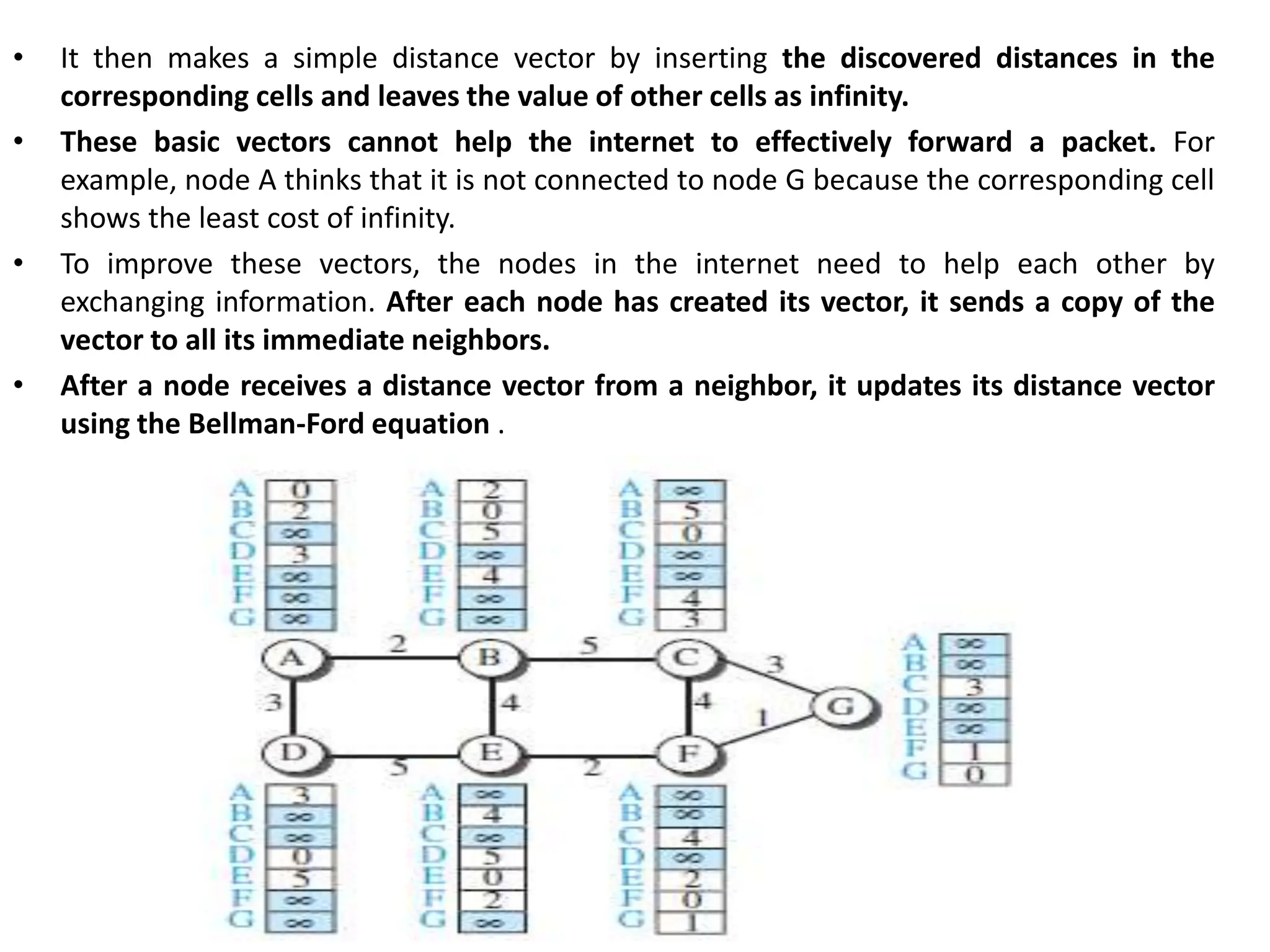
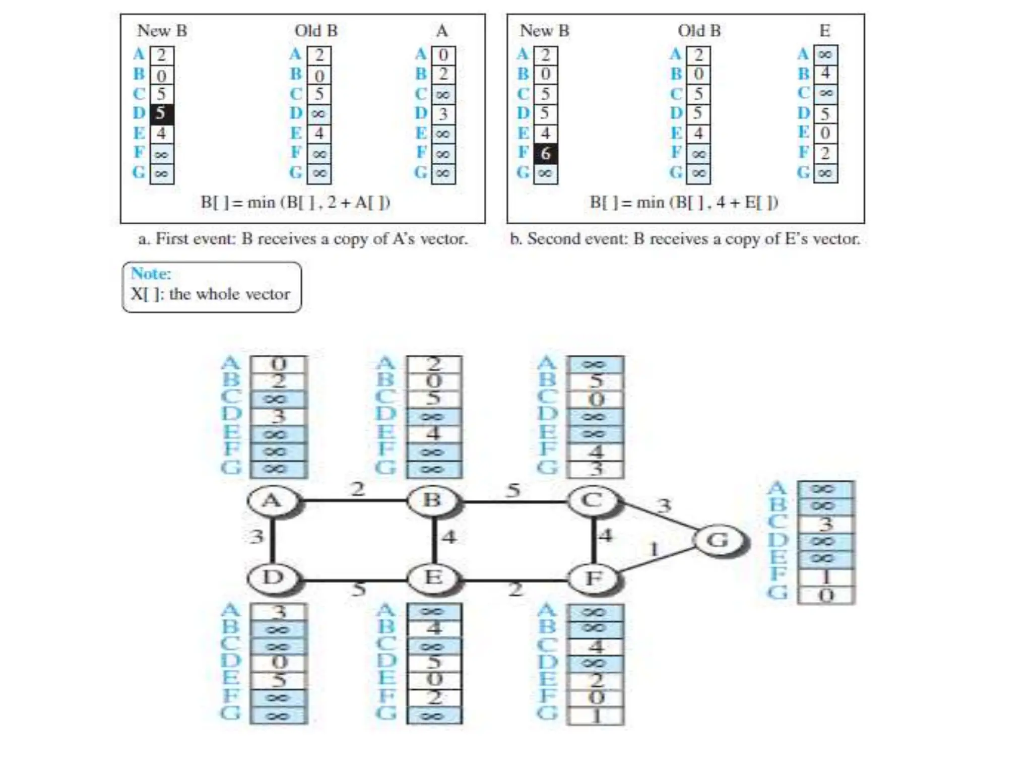
Distance-Vector Routing Algorithm
Distance_Vector_Routing ( )
{
// Initialize (create initial vectors for the node)
D[myself ] = 0
for (y = 1 to N)
{
if (y is a neighbor)
D[y] = c[myself ][y]
else
D[y] = ∞
}
send vector {D[1], D[2], …, D[N]} to all neighbors
// Update (improve the vector with the vector received from a neighbor)
repeat (forever) {
wait (for a vector Dw from a neighbor w or any change in the link)
for (y = 1 to N) {
D[y] = min [D[y], (c[myself ][w] + Dw[y ])] // Bellman-Ford equation
}
if (any change in the vector)
send vector {D[1], D[2], …, D[N]} to all neighbors }
} // End of Distance Vector

DVR Problem
• For the network given above, give the global distance vector tables when
using Distance Vector Routing Algorithm for the following three instances.
• a. Each node knows only the distances to its immediate neighbours.
• b. Each node has reported the information it had in the preceding step to
its immediate neighbours.
• c. Step (b) happens a second time.

2. Link State Routing
• The term link-state is to define the characteristic of a link (an edge) that
represents a network in the internet.
• In this algorithm, the cost associated with an edge defines the state of the link.
Link-State Database (LSDB)
• Each node needs to have a complete map of the network, which means it
needs to know the state of each link.
• The collection of states for all links is called the link-state database (LSDB).
• There is only one LSDB for the whole internet; each node needs to have a
duplicate of it to be able to create the least-cost tree.
• The LSDB can be represented as a two-dimensional array (matrix) in which the
value of each cell defines the cost of the corresponding link.

Computer Networks 22-119
Link State Routing
• Each node has the entire topology of the domain- the list of nodes and links, how
they are connected including type, cost, and condition of the links(up or down)
• Node can use Dijkstra’s algorithm to build a routing table

Flooding
• Each node can create this LSDB that contains information about the whole
internet. This can be done by a process called flooding.
• Each node can send some greeting messages to all its immediate
neighbors (those nodes to which it is connected directly) to collect two
pieces of information for each neighboring node: the identity of the node
and the cost of the link.
• The combination of these two pieces of information is called the LS packet
(LSP); the LSP is sent out of each interface.

121
Operation of a Link State Routing
protocol
Received
LSAs
IP Routing
Table
Dijkstra’s
Algorithm
Link State
Database
LSAs are flooded
to other interfaces

Figure. LSPs created and sent out by each node to build LSDB
Routing Table Creation
1. Creation of the states of the links by each node, called the link state packet (LSP)
2. Dissemination of LSPs to every other router, called flooding, in an efficient and reliable way
3. Formation of a shortest path tree for each node
4. Calculation of a routing table based on the shortest path tree
Flooding of LSPs
1. The creating node sends a copy of the LSP out of each interface
2. A node compares it with the copy it may already have. If the newly arrived LSP is older than
the one it has, it discards the LSP. If it is newer,
 It discards the old LSP and keeps the new one
 It sends a copy of it out of each interface except the one from which the packet arrived

Comparison
• In the distance-vector routing algorithm, each
router tells its neighbors what it knows about
the whole internet.
• In the link-state routing algorithm, each router
tells the whole internet what it knows about
its neighbors.

Formation of Least-Cost Trees
• To create a least-cost tree for itself, using the shared LSDB, each node
needs to run the famous Dijkstra Algorithm. This iterative algorithm uses
the following steps:
1. The node chooses itself as the root of the tree, creating a tree with a single
node, and sets the total cost of each node based on the information in the
LSDB.
2. The node selects one node, among all nodes not in the tree, which is
closest to the root, and adds this to the tree. After this node is added to
the tree, the cost of all other nodes not in the tree needs to be updated
because the paths may have been changed.
3. The node repeats step 2 until all nodes are added to the tree.

Figure Forming shortest path three for router A in a graph

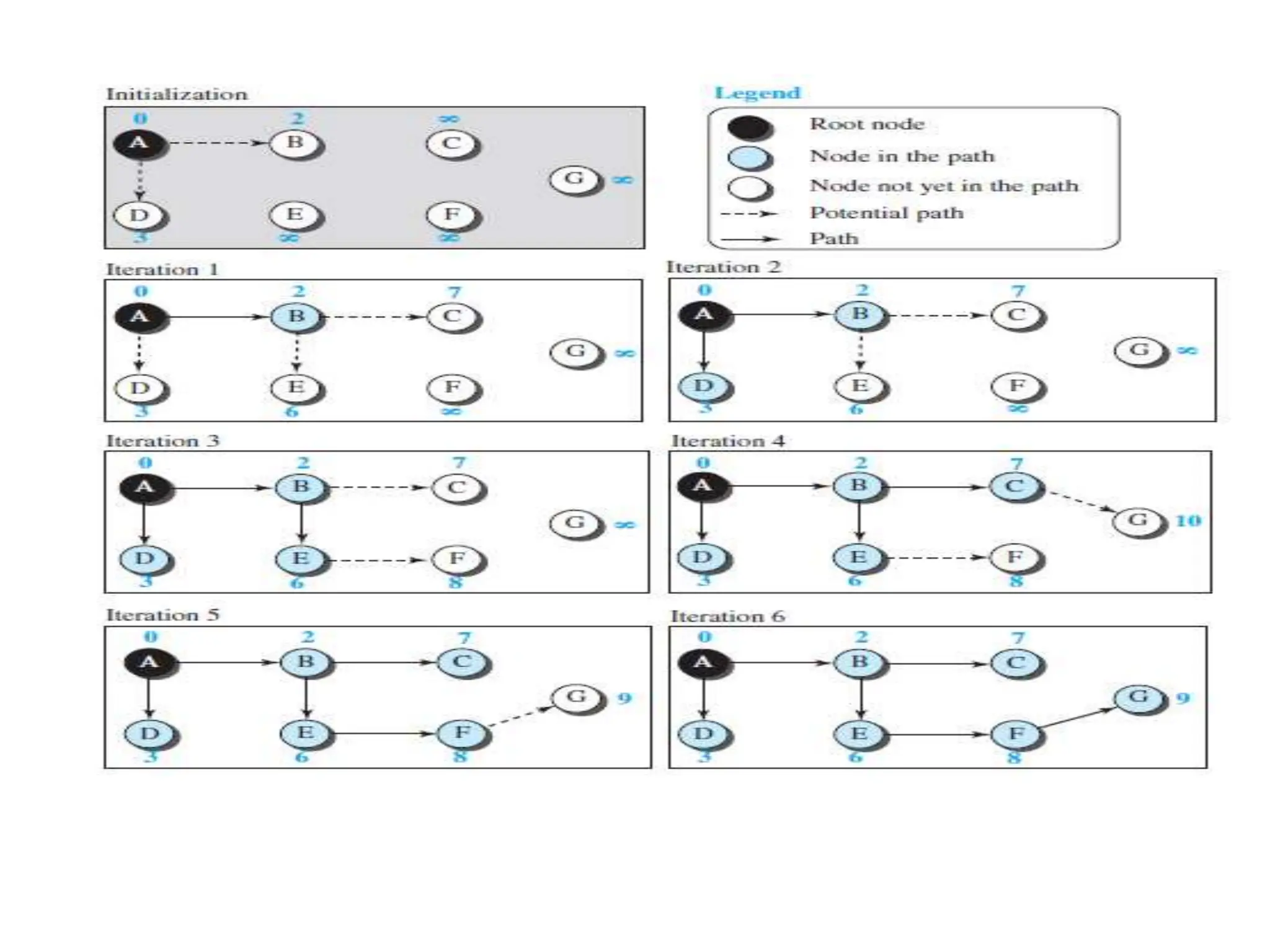
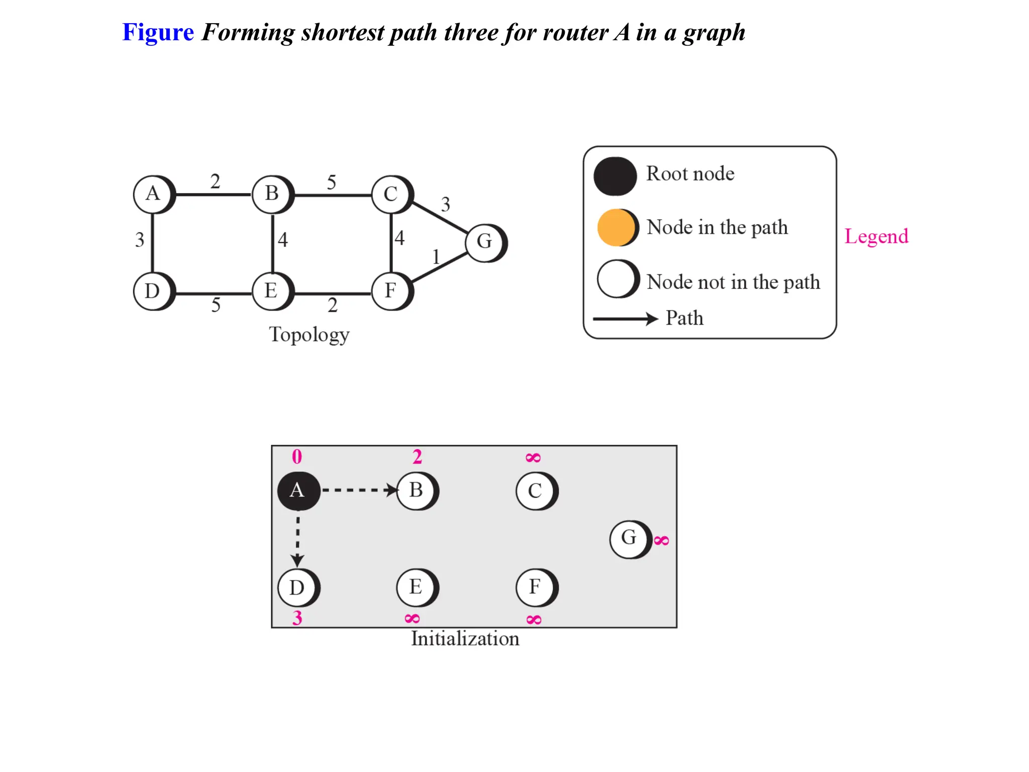
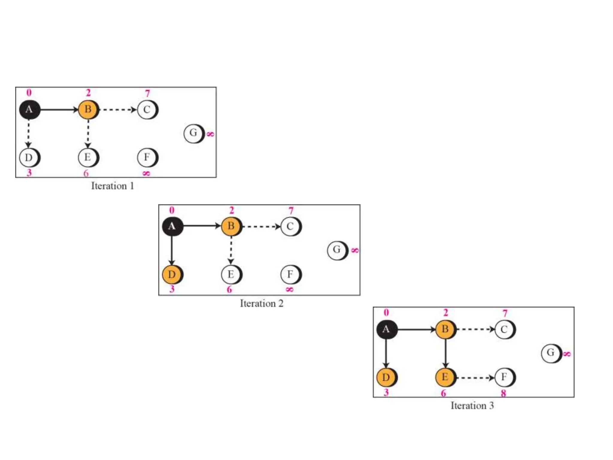
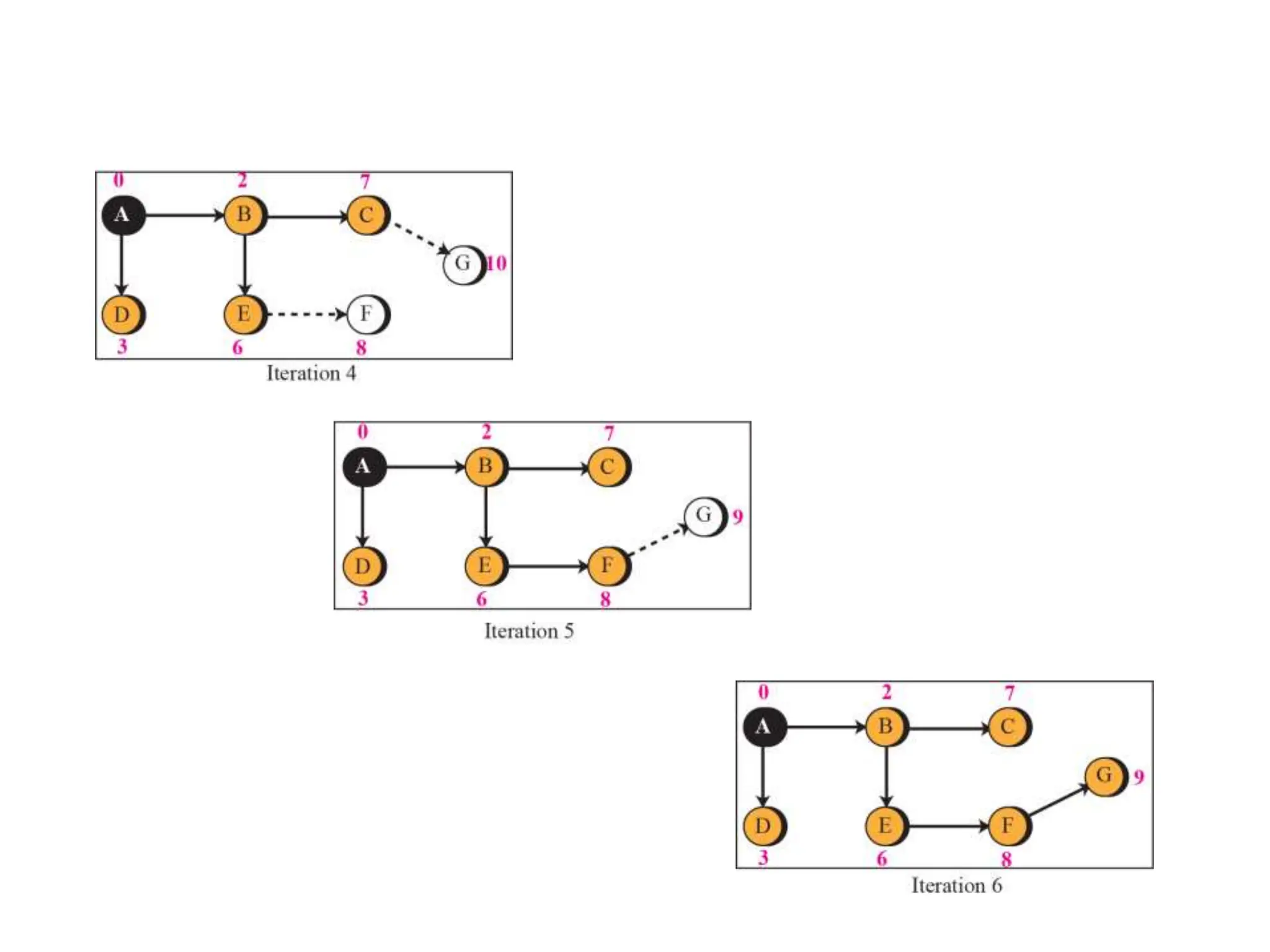
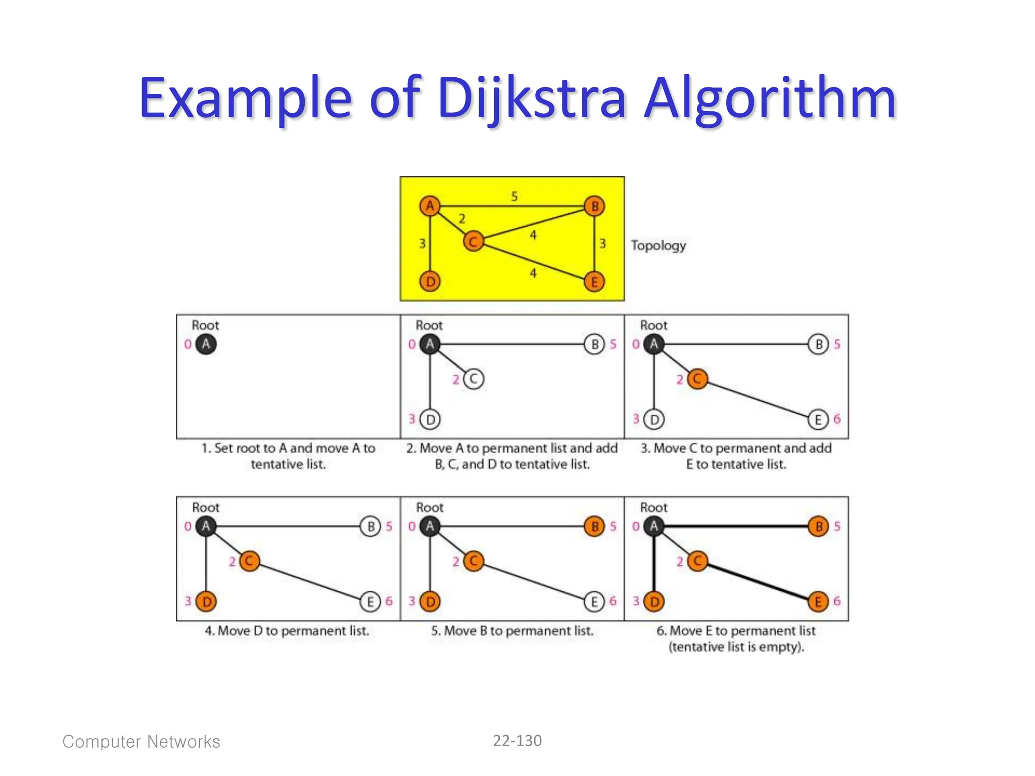
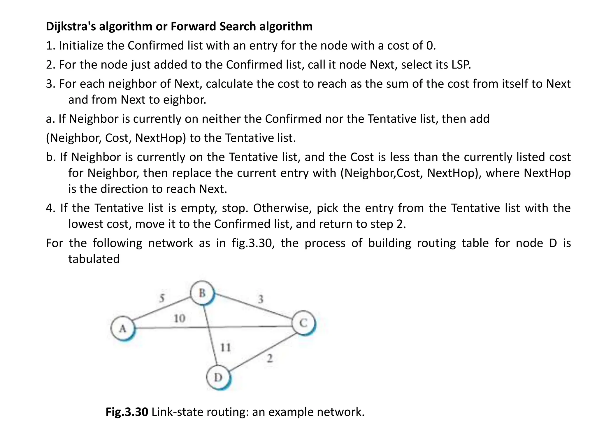
Dijkstra’s Algorithm ( )
{
// Initialization
Tree = {root} // Tree is made only of the root
for (y = 1 to N) // N is the number of nodes
{
if (y is the root)
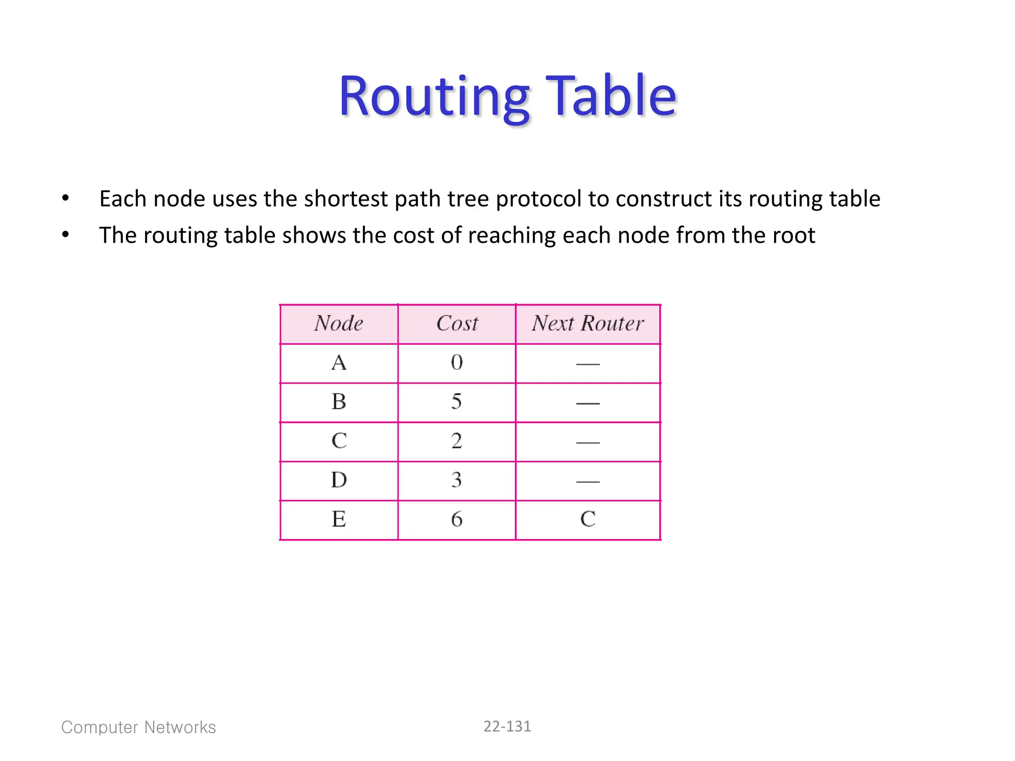
D[y] = 0 // D[y] is shortest distance from root to node y
else if (y is a neighbor)
D[y] = c[root][y] // c[x][y] is cost between nodes x and y in LSDB
else
D[y] = ∞
}
// Calculation
repeat {
find a node w, with D[w] minimum among all nodes not in the Tree
Tree = Tree ∪ {w} // Add w to tree
// Update distances for all neighbors of w
for (every node x, which is a neighbor of w and not in the Tree)
{
D[x] = min{D[x], (D[w] + c[w][x])} }
} until (all nodes included in the Tree)
} // End of Dijkstra

Example of Dijkstra Algorithm

Routing Table
• Each node uses the shortest path tree protocol to construct its routing table
• The routing table shows the cost of reaching each node from the root

Routing Information Protocol (RIP)
• Routing Information Protocol (RIP) is the canonical example of a routing protocol built on the
distance-vector algorithm.
• RIP is an intra-domain routing protocol used inside an autonomous system(An autonomous
system (AS) is a network or a collection of networks that are all managed and supervised by a
single entity or organization).
• It is extremely simple and widely used.
• The routers advertise the cost of reaching networks, instead of reaching other routers.
• Consider the following network
Fig.3.27 Example network running RIP
• In fig.3.27, Router C advertises to router A that it can reach networks 2 and 3 at a cost of 0,
networks 5 and 6 at cost 1 and network 4 at cost 2.
• RIP takes the simplest approach, with all link costs being equal to 1.
• The distance is defined as the number of links to reach the destination. The metric in RIP is
called a hop count.
• Infinity is defined as 16, i.e., any route in an AS using RIP cannot have more than 15 hops. It is
limited to run on only smaller networks.
• Routers running RIP send their advertisements every 30 seconds.

Packet Format
• The RIP packet format is given below. The majority of the
packet is taken up with (network-address, distance) pairs.
Fig.3.28 RIP packet format

Link State (OSPF)
Link-state routing protocols rely on two mechanisms:
1. Reliable dissemination of link-state information
2. Calculation of routes from all the accumulated link-state knowledge
Reliable Flooding
• Reliable flooding is the process of ensuring all nodes having a copy of the
link-state information from all the other nodes
• Each node creates an update packet called a link-state packet (LSP) that
contains
– ID of the node
– List of directly connected neighbors of that node and the cost to each one
– Sequence number
– Time to live(TTL)for this packet
• Transmission of LSPs between adjacent routers is made reliable using
acknowledgments.
• Each node that receives a LSP checks to see whether it has a copy.
– If not, it stores and forwards the LSP on all of its links
– If it has a copy, it compares the sequence numbers.
• If the received LSP has a bigger sequence number, then it is stored and
forwarded, since it is a recent LSP. The old one discarded.

• Since a node passes a recent LSP to its neighbors and who in turn forward it their neighbors,
the recent LSP eventually reaches all nodes.
• LSP is generated either periodically or when there is a change in the topology detected using
hello packets.
• In fig.3.29, each node sends its LSP out on each of its directly connected links.
• LSP arrives at node X, which sends it to neighbors A and C. A and C do not send it back to X, but
send it on to B.
• Consider the flooding in a small network
Fig.3.29 Flooding of link-state packets. (a) LSP arrives at node X ;(b) X floods LSP to A and C;(c) A
and C flood LSP to B;(d) flooding is complete.
• Since B receives two identical copies of the LSP, it will accept whichever arrived first and ignore
the second as a duplicate.
• It then passes the LSP on to D. Since D has no neighbors to flood the process is complete.

Reducing Overhead
• Flooding creates traffic and is an overhead to the network.
Mechanisms to reduce are:
• Timers ->using long timers, in terms of hours for periodic generation.
• Sequence numbers ->64-bit sequence numbers ensure that they do not
wrap around so soon and is used to discard old LSPs.
• Time to live-> A router always decrements TTL before forwarding a LSP.
When the TTL reaches 0, the node refloods the LSP with a TTL of 0, to
which all the nodes in the network delete that LSP.
Route Calculation
• Once a node has copy of the LSP from every other node, it knows the
entire network.
• Each node computes its routing table directly from the LSPs using a
realization of Dijkstra's algorithm is called forward search algorithm.
• Each node maintains two lists namely Tentative and Confirmed.
• Each of these lists contains a set of entries of the form (Destination, Cost,
NextHop)

Dijkstra's algorithm or Forward Search algorithm
1. Initialize the Confirmed list with an entry for the node with a cost of 0.
2. For the node just added to the Confirmed list, call it node Next, select its LSP.
3. For each neighbor of Next, calculate the cost to reach as the sum of the cost from itself to Next
and from Next to eighbor.
a. If Neighbor is currently on neither the Confirmed nor the Tentative list, then add
(Neighbor, Cost, NextHop) to the Tentative list.
b. If Neighbor is currently on the Tentative list, and the Cost is less than the currently listed cost
for Neighbor, then replace the current entry with (Neighbor,Cost, NextHop), where NextHop
is the direction to reach Next.
4. If the Tentative list is empty, stop. Otherwise, pick the entry from the Tentative list with the
lowest cost, move it to the Confirmed list, and return to step 2.
For the following network as in fig.3.30, the process of building routing table for node D is
tabulated
Fig.3.30 Link-state routing: an example network.

Table: 3.5 Steps for building routing table for node D
B
A
D
C
5 3
2
11
10

• Given the network topology below, use a link-state algorithm to compute the shortest path from A to all
other nodes. Make sure to show the result of the computation at each step.(Apr/May 2008)
B D
A C
E
7
12 1
10
1
3
1

Open Shortest Path First Protocol (OSPF)
Open Shortest Path First Protocol (OSPF) is one of the
most widely used link-state routing protocols.
The features added to link-state algorithm are:
1. Authentication of routing messages: Misconfigured
hosts are capable of bringing down a network by
advertising to reach every host with the lowest cost 0.
Such disasters are prevented by mandating routing
updates to be authenticated.
2. Additional hierarchy: In OSPF, a domain is partitioned
into areas, i.e., a router need not know the complete
network, instead only its area.
3. Load balancing: OSPF allows multiple routes to the
same place to be assigned the same cost and will cause
traffic to be distributed evenly over those routes

OSPF Header
OSPF header fields are shown in fig.3.31, they are
Version -represents the current version, i.e., 2.
Type- represents the type value (1-5) of OSPF message.
SourceAddr -identifies the sender of the message
AreaId- 32-bit identifier of the area in which the node is located
Checksum-16-bit checksum
Authentication type -has value 0 if no authentication is used, 1 for simple password and 2 for
cryptographic authentication checksum.
Authentication(system verifies the identity of a user) -contains password or cryptographic checksum
Fig.3.31 OSPF header format
Note: The art of protecting information by transforming it (encrypting it) into an unreadable format

Link-state Advertisement fields are as follows:
LS Age-similar to TTL is incremented at each node until it reaches a maximum (expiry)
Type- defines type of LSA. Type1 LSAs advertise the cost of links between routers.
Link-state ID -32-bit identifier of the router.
Advertising router- For type 1 LSA, it is same as Link-state ID
LS sequence number- used to detect old or duplicate packets
LS checksum- covers all fields except LS Age
Length- length of the LSA in bytes
Link ID and Link Data- identify a link
Metric- specifies cost of the link.
Type- specifies type of link (for example, point-to-point)
TOS- allows OSPF to choose different routes based on the value in TOS field.
Fig.3.32 Link-state Advertisement

Difference between ipv4 and ipv6
IPv4 Address IPv6 Address
Address Length – 32 bits 128 bits
Address Representation - decimal hexadecimal
Internet address classes Not applicable in IPv6
Multicast addresses (224.0.0.0/4) IPv6 multicast addresses (FF00::/8)
Broadcast addresses Not applicable in IPv6
Unspecified address is 0.0.0.0 Unspecified address is ::
Public IP addresses Global unicast addresses
Private IP addresses (10.0.0.0/8, 172.16.0.0/12,
and 192.168.0.0/16)
Site-local addresses (FEC0::/10)
Autoconfigured addresses (169.254.0.0/16) Link-local addresses (FE80::/64)
Text representation: Dotted decimal notation Text representation: Colon hexadecimal format
with suppression of leading zeros and zero
compression. IPv4-compatible addresses are
expressed in dotted decimal notation.
Network bits representation: Subnet mask in
dotted decimal notation or prefix length
Network bits representation: Prefix length notation
only

IPv6 ADDRESSES
• Despite all short-term solutions, such as classless addressing, Dynamic Host
Configuration Protocol (DHCP), NAT, address depletion is still a long-term problem
for the Internet.
• Other problems in the IP protocol itself, such as lack of accommodation for real-
time audio and video transmission, and encryption and authentication of data
for some applications, have been the motivation for IPv6.
Figure.3.10 IPv6 address in binary and hexadecimal colon notation

Hexadecimal Colon Notation
• To make addresses more readable, IPv6 specifies hexadecimal colon
notation. In this notation, 128 bits is divided into eight sections, each 2
bytes in length.
• Two bytes in hexadecimal notation requires four hexadecimal digits.
Therefore, the address consists of 32 hexadecimal digits, with every four
digits separated by a colon, as shown in Figure.
Figure.3.11 Abbreviated IPv6 addresses
Abbreviation
• Although the IP address, even in hexadecimal format, is very long, many
of the digits are zeros.
• In this case, we can abbreviate the address. The leading zeros of a section
(four digits between two colons) can be omitted.

Example-16
Expand the address 0:15:: 1:12:1213 to its original.
Solution:
We first need to align the left side of the double colon to the left of the original
pattern and the right side of the double colon to the right of the original pattern to
find how many 0s we need to replace the double colon.
Thismeansthattheoriginaladdressis.

Address Space
• IPv6 has a much larger address space; 2128 addresses are
available. The designers of IPv6 divided the address into
several categories.
• A few leftmost bits, called the type prefix, in each address
define its category. The third column shows the fraction of
each type of address relative to the whole address space.
Type prefixes for IPv6 addresses

Unicast Addresses
• A unicast address defines a single computer. The packet sent to a unicast address must be
delivered to that specific computer.
• IPv6 defines two types of unicast addresses: geographically based and provider-based. The
first type is left for future definition.
• The provider-based address is generally used by a normal host as a unicast address. The
address format is shown in Figure.
• Fields for the provider-based address are Type identifier, Registry identifier, Provider
identifier, Subscriber identifier, Subnet identifier and Node identifier.
Fig. Prefixes for provider-based unicast address

Multicast Addresses
• Multicast addresses are used to define a group of hosts instead of just one. A packet sent to a
multicast address must be delivered to each member of the group. Figure. shows the format of
a multicast address.
Figure.3.12 Multicast address in IPv6
• The second field is a flag that defines the group address as either permanent or transient.
• A permanent group address is defined by the Internet authorities and can be accessed at all
times. A transient group address, on the other hand, is used only temporarily.
Any cast Addresses
• IPv6 also defines anycast addresses.
• An anycast address, like a multicast address, also defines a group of nodes. However, a packet
destined for an anycast address is delivered to only one of the members of the anycast group,
the nearest one (the one with the shortest route).
• Although the definition of an anycast address is still debatable, one possible use is to assign an
anycast address to all routers of an ISP that covers a large logical area in the Internet.
• The routers outside the ISP deliver a packet destined for the ISP to the nearest ISP router. No
block is assigned for anycast addresses.

Reserved Addresses
• Another category in the address space is the reserved address. These addresses
start with eight 0s (type prefix is 00000000).
Figure.3.13 Reserved addresses in IPv6
• An unspecified address is used when a host does not know its own address and
sends an inquiry to find its address.
• A loopback address is used by a host to test itself without going into the network.
• A compatible address is used during the transition from IPv4 to IPv6.
• A mapped address is also used during transition. However, it is used when a
computer that has migrated to IPv6 wants to send a packet to a computer still
using IPv4.

Local Addresses
• These addresses are used when an organization wants to use IPv6 protocol
without being connected to the global Internet. In other words, they
provide addressing for private networks.
• Nobody outside the organization can send a message to the nodes using
these addresses. Two types of addresses are defined for this purpose.
• A link local address is used in an isolated subnet; a site local address is
used in an isolated site with several subnets.
Figure.3.14 Local Addresses in IPv6

(Internetworking Protocol, version 6 )IPv6
• IPv4 has some deficiencies that make it unsuitable for the fast-growing Internet. Address
depletion is still a long-term problem in the Internet.
• The Internet must accommodate real-time audio and video transmission. This type of
transmission requires minimum delay strategies and reservation of resources not provided
in the IPv4 design.
• No encryption or authentication is provided by IPv4.
• To overcome these deficiencies, IPv6 (Internetworking Protocol, version 6), also known as
IPng (Internetworking Protocol, next generation), was proposed and is now a standard.
Advantages of IPv6
₋ Larger address space
₋ Better header format
₋ New options
₋ Allowance for extension
₋ Support for resource allocation
₋ Support for more security
Packet Format
• The IPv6 packet is shown in Figure. Each packet is composed of a mandatory base header
followed by the payload.
• The payload consists of two parts: optional extension headers and data from an upper layer.
• The base header occupies 40 bytes, whereas the extension headers and data from the
upper layer contain up to 65,535 bytes of information.

Base Header
Figure. shows the base header with its eight fields.
These fields are as follows:
Version. This 4-bit field defines the version number of
the IP. For IPv6, the value is 6.
Priority. The 4-bit priority field defines the priority of
the packet with respect to traffic congestion.
Figure.IPv6 datagram header and payload

Figure. Format of an IPv6 datagram
Flow label. The flow label is a 3-byte (24-bit) field that is designed to provide special
handling for a particular flow of data.
Payload length. The 2-byte payload length field defines the length of the IP datagram
excluding the base header.
Next header. The next header is an 8-bit field defining the header that follows the
base header in the datagram.
Hop limit. This 8-bit hop limit field serves the same purpose as the TTL field in IPv4.
Source address. The source address field is a 16-byte (128-bit) Internet address that
identifies the original source of the datagram.
Destination address. The destination address field is a 16-byte (128-bit) Internet
address that usually identifies the final destination of the datagram.
Priority The priority field of the IPv6 packet defines the priority of each packet with
respect to other packets from the same source.

Extension Headers
• The length of the base header is fixed at 40 bytes. However, to give greater
functionality to the IP datagram, the base header can be followed by up to six
extension headers.
• Many of these headers are options in IPv4. Six types of extension headers have been
defined.
• They are Hop-by-hop option, Source routing, Fragmentation, Authentication,
Encrypted security payload, Destination option.
Comparison between IPv4 and IPv6 Headers
1. The header length field is eliminated in IPv6 because the length of the header is fixed
in this version.
2. The service type field is eliminated in IPv6. The priority and flow label fields together
take over the function of the service type field.
3. The total length field is eliminated in IPv6 and replaced by the payload length field.
4. The identification, flag, and offset fields are eliminated from the base header in IPv6.
They are included in the fragmentation extension header.
5. The TTL field is called hop limit in IPv6.
6. The protocol field is replaced by the next header field.
7. The header checksum is eliminated because the checksum is provided by upper-layer
protocols; it is therefore not needed at this level.
8. The option fields in IPv4 are implemented as extension headers in IPv6.

FORWARDING OF IP PACKETS
• Forwarding means to place the packet in its route to
its destination.
• Since the Internet today is made of a combination of
links (networks), forwarding means to deliver the
packet to the next hop (which can be the final
destination or the intermediate connecting device).
• When IP is used as a connectionless protocol,
forwarding is based on the destination address of the
IP datagram;
• when the IP is used as a connection-oriented
protocol, forwarding is based on the label attached
to an IP datagram.

Forwarding Based on Destination Address
• In this case, forwarding requires a host or a router to have a
forwarding table.
• When a host has a packet to send, it looks at this table to find
the next hop to deliver the packet to.
• In classless addressing, the whole address space is one entity;
there are no classes.
• The table needs to be searched based on the network address
(first address in the block).
• Unfortunately, the destination address in the packet gives no
clue about the network address.
• To solve the problem, we need to include the mask (/n) in the
table. In other words, a classless forwarding table needs to
include four pieces of information: the mask, the network
address, the interface number, and the IP address of the next
router.

Simplified forwarding module in classful address
with subnetting

TCP/IP Protocol Suite 162
In classful addressing we can have a
routing table with three columns;
in classless addressing,
we need at least four columns.
Note

Fig. Simplified forwarding module in classless address
• The job of the forwarding module is to search the table, row by row.
• In each row, the n leftmost bits of the destination address (prefix) are kept and the
rest of the bits (suffix) are set to 0s.
• If the resulting address (which we call the network address), matches with the
address in the first column, the information in the next two columns is extracted;
otherwise the search continues.

• Longest Mask Matching
• This principle states that the forwarding table is sorted from the longest
mask to the shortest mask. In other words, if there are three masks, /27,
/26, and /24, the mask /27 must be the first entry and /24 must be the
last. Let us see if this principle solves the situation in which organization 4
is separated from the other three organizations.
• Hierarchical Routing
• To solve the problem of gigantic forwarding tables, we can create a sense
of hierarchy in the forwarding tables. Internet is divided into backbone
and national ISPs. National ISPs are divided into regional ISPs, and regional
ISPs are divided into local ISPs. If the forwarding table has a sense of
hierarchy like the Internet architecture, the forwarding table can decrease
in size.
• Inside the local ISP, the router must recognize the subblocks and route the
packet to the destined customer. If one of the customers is a large
organization, it also can create another level of hierarchy by subnetting
and dividing its subblock into smaller subblocks (or sub-subblocks). In
classless routing, the levels of hierarchy are unlimited as long as we follow
the rules of classless addressing.

• Geographical Routing
• To decrease the size of the forwarding table even further, we need to extend
hierarchical routing to include geographical routing. We must divide the entire
address space into a few large blocks. We assign a block to America, a block to
Europe, a block to Asia, a block to Africa, and so on. The routers of ISPs outside of
Europe will have only one entry for packets to Europe in their forwarding tables.
The routers of ISPs outside of America will have only one entry for packets to
America in their forwarding tables, and so on.
• Forwarding Table Search Algorithms
• In classless addressing, there is no network information in the destination
address. The simplest, but not the most efficient, search method is called the
longest prefix match. The forwarding table can be divided into buckets, one for
each prefix. The router first tries the longest prefix. If the destination address is
found in this bucket, the search is complete. If the address is not found, the next
prefix is searched, and so on. It is obvious that this type of search takes a long
time. One solution is to change the data structure used for searching. Instead of a
list, other data structures (such as a tree or a binary tree) can be used. One
candidate is a trie (a special kind of tree).

• Forwarding Based on Label
• In the 1980s, an effort started to somehow change IP to behave like a connection
oriented protocol in which the routing is replaced by switching. In a connectionless
network (datagram approach), a router forwards a packet based on the destination
address in the header of the packet. On the other hand, in a connection-oriented
network (virtual-circuit approach), a switch forwards a packet based on the label
attached to the packet. Routing is normally based on searching the contents of a
table; switching can be done by accessing a table using an index. In other words,
routing involves searching; switching involves accessing.
• Multi-Protocol Label Switching (MPLS)
• During the 1980s, several vendors created routers that implement switching
technology. Later IETF approved a standard that is called Multi-Protocol Label
Switching. In this standard, some conventional routers in the Internet can be
replaced by MPLS routers, which can behave like a router and a switch. When
behaving like a router, MPLS can forward the packet based on the destination
address; when behaving like a switch, it can forward a packet based on the label.

• A New Header
• To simulate connection-oriented switching using a protocol like IP, the first thing that is
needed is to add a field to the packet. The IPv4 packet format does not allow this extension.
The solution is to encapsulate the IPv4 packet in an MPLS packet (as though MPLS were a
layer between the data-link layer and the network layer). The whole IP packet is encapsulated
as the payload in an MPLS packet and an MPLS header is added.
• Hierarchical Switching
• A stack of labels in MPLS allows hierarchical switching. This is similar to conventional
hierarchical routing. For example, a packet with two labels can use the top label to forward
the packet through switches outside an organization; the bottom label can be used to route
the packet inside the organization to reach the destination subnet.
• Routers as Packet Switches
• The packets switches are used in the network layer are called routers. Routers can be
configured to act as either a datagram switch or a virtual-circuit switch.

• https://forms.gle/1NJbwGwqrWTdYxxF7

UNIT-3 network security layers andits types

Recommended

Recommended

More Related Content

Similar to UNIT-3 network security layers andits types

Similar to UNIT-3 network security layers andits types (20)

Recently uploaded

Recently uploaded (20)

UNIT-3 network security layers andits types